Category: Cloud Software

Let’s build a lightweight stock tracker in Google Sheets using the GOOGLEFINANCE function. The GOOGLEFINANCE function brings current and historical securities data into Google Sheets, eliminating the need to use connections to outside financial services.

There are plenty of complicated stock trackers, but that’s not what this is. It’s a learning tool. We’re building this tracker to learn about the GOOGLEFINANCE function, special characters, and charts. So, let’s get started!

You have $50,000 to invest, and you want to find some stocks for a long-term investment.

Retrieving Current Stock Data with GOOGLEFINANCE

Let’s start with retrieving current data, and we’ll use four well-known stocks for the comparison – General Electric, Microsoft, PPG, and US Steel. We’ll build a table with these ticker symbols as the rows and price, price-to-earnings (pe), and beta as the column headers. Although it’s not required, the function prefers we prepend the ticker symbols with their stock exchange to be more precise. Therefore, GE will become NYSE:GE and MSFT will be NASDAQ:MSFT, etc.

Retrieving Stock Price with GOOGLEFINANCE

Column B will be the security’s current price. Before we write the formula in this column, let’s examine its syntax.

=GOOGLEFINANCE(ticker symbol, [attribute], [start_date], [end_date|num_days], [interval])

As you can see, the only required argument is the ticker symbol. Using just the ticker symbol will retrieve the current price. Let’s do that for this first column of stock data. Since we have the securities listed in A2:A5, we can reference those in the formulas. In cell B2, we’ll use the sytnax of =GOOGLEFINANCE($A2).

Notice the $ before the A in the cell reference. This fixes the reference to column A. When we drag the formulas to the right for the other attributes, the column reference won’t change.

Drag the formula in B2 down through B5. Now we have our stock prices.

Retrieving the P/E Ratio with GOOGLEFINANCE

Next, let’s look up the price-to-earnings ratio. The price-to-earnings ratio is a good measure of a company’s relative profitability. In the previous example, the only input for the GOOGLEFINANCE function was the stock exchange and ticker symbol. Now we need to specify the attribute of “pe” in column C. Let’s do this using a cell reference.

Drag the formula from cell B2 into C2 and you’ll get this: =GOOGLEFINANCE($A2). This fixed cell reference worked; otherwise, the cell reference would have been B2. Now, we need to add the attribute of pe. We’ll do that by referencing cell C1 and fixing the row number with a $ so it can be copied down without changing.

The completed formula for GE’s pe is =GOOGLEFINANCE($A2,C$1).

If you’re observant, you’ll notice the result is an error. This is because GE has not had positive earnings recently (it’s now early 2023); therefore, there are no earnings for the calculation. However, we see results when we copy the formula down for the other ticker symbols.

That covers the price-to-earnings ratio. Let’s move on to our next attribute.

Retrieving Beta with GOOGLEFINANCE

Let’s repeat the process for the beta attribute. A stock’s beta is a measure of its volatility.

The formula for GE’s beta is – =GOOGLEFINANCE($A2,D$1).
Because we fixed the column reference for the ticker symbol and the row reference for the attribute, we can complete these formulas without typing.

After dragging the formulas down and over, we have a completed table of current stock data.

Retrieving Hisotrical Stock Data with GOOGLEFINANCE

Now let’s take a look at the historical data that’s available.

If I picked individual stocks myself, which I don’t, I would be most interested in historical performance measures. Items such as historical price-to-earnings, return-on-assets, and profit margin percentage would be a good place to start. However, the historical data for stocks is limited to share price data. Let’s make the most with what we have.

We will look at share price over time, then visualize it with a chart and custom number formatting. Let’s start with a basic grid to hold our data.

Since we discussed the basics of the GOOGLEFINANCE function previously, we’ll skip that part and jump into what’s different this time.

Formula to be used in cell B2: =INDEX(GOOGLEFINANCE($A2,"close",B$1),2,2)

There are a few new things about this formula. The first is the addition of the start_date, which is the cell reference B$1. The function needs a start_date when retrieving historical data.

The second change is that the attribute is typed directly into the formula instead of retrieved with a cell reference. We are using close this time, which is the closing stock price on the given start_date.

The third addition to the formula is a function called INDEX. INDEX fetches and returns part of an array. The function is needed here because GOOGLEFINANCE returns four cells of data when retrieving a historical stock price. We’ll trim these four cells down to one. The INDEX function needs the row and column numbers, which in this case are 2 and 2.

After using the INDEX function, we have only stock price, which is the result from the second column and second row of the output from the GOOGLEFINANCE function.

Conclusion of Setting Up Data

Now that we know how to build each formula, we’ll paste them into the empty grid.

Each year’s closing price is helpful, but it’s the year-over-year change in that price that we’re after. We’ll do some simple arithmetic in each “% change” cell so show how much each stock price rose or fell.

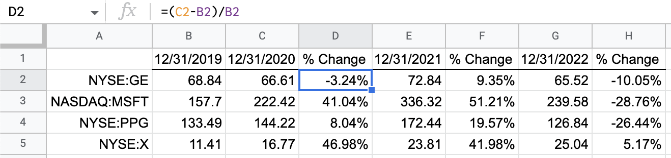
Year over year change formula in cell D2 – =(C2-B2)/B2

Now we have all the data we need to create visualizations to help us understand the data. We’ll dive into these graphs and special characters in this next post.