If you want to track your employees’ time, there is an easy way to do it using Google Sheets that does not involve complicated formulas or macros. This technique will also have the ability to calculate an overnight shift. The linked file that can be copied into your own Drive and used as a template.
Data validation
One of the most difficult things when working with dates and time in Sheets is getting them in the cells correctly. A protection against that, data validation, can be used to reject invalid inputs.
Click on the Data menu option and then Data Validation.

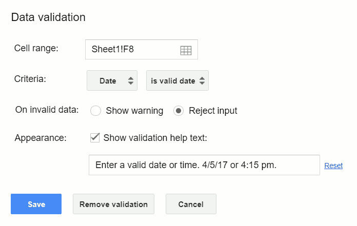
Once the Data validation window pops up, complete it with the parameters in the following pictures including choosing Date from the criteria drop-down box and rejecting invalid input with a message.

This will set data validation to show the message “Enter a valid date or time” if an invalid date is entered. Times are covered under the date formatting as card card-body bg-light so this data validation is also going to work if it’s a time. Now, if a user enters a date or time that Sheets doesn’t recognize as such, they will get an error message letting them know. There are several different ways to enter a date using a valid format, but there’s infinitely more ways to screw it up. You could do 2-20-18. You could type out February. But, as long as it’s valid, this timesheet will accept it.
The same thing is going to happen with time. If it’s 5:43 and the person types 5 43 in hits enter, it’s not going to work. You have to have a number, a colon, and a number. If you want seconds, do another colon and two digits after that such as 5:43:22.
The formula
Once the validation of the dates and times is set up correctly, the spreadsheet is ready for a start day and time and an end day and time. This formula is going to calculate the hours. So this formula is going to look a little complicated at first, but it’s really not too bad.
Copy and paste this code for column D
=((DATEVALUE(B5)+TIMEVALUE(C5)-(DATEVALUE(B4)+TIMEVALUE(C4)))*24)

As seen in the shared sheet, this formula takes the row it is on and subtracts it from the row above it. To do arithmetic with these dates and times, Sheets has to convert them into a value first. That is what the DATEVALUE and TIMEVALUE functions are doing. The result will be a fraction of a day so multiply that by 24 and that gives you the number of hours worked. Every other row, you want to put in this formula.
If this person takes breaks, just repeat the same formula. If you want to make this longer, just copy and paste it down as many times as you want.
To find durations for longer periods, use the TIMEDIF add-on. It outputs years, months, weeks, days, hours, and more.
Conclusion
After following this tutorial, you should be able to create a time sheet to track the hours of your empoyees. If you have any questions, feel free to leave a comment below.
Alice Kelly says:
Thanks for this but I need to create one with a couple of ins and out times within each day. I can’t find any tutorial for this.
Prolific Oaktree says:
You could use as many rows as you want and just copy and paste them as you go.
tamie bateman says:
Thank you for this information, I learned a lot and it is so helpful. I need to add a lunch break in this and still have it calculate the hours, how do I do that?
Prolific Oaktree says:
I would just treat it as a new entry below the previous one.
shawn wood says:
how can I total the column? the sum function just goves me a #value… thanks in advance.
Prolific Oaktree says:
There must be some non numbers in the row. Use the ISNUMBER function on each value to check.
Chris Whited says:
This work great but is there any way to make the time automatic. Like double click in the box and it fill out the current time?
Prolific Oaktree says:
See this video about timestamps. I’m not sure if it always works though;) https://youtu.be/cQmNX5ATxB0