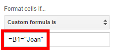
Highlighting Just One Cell
Right now, our custom formula that we built in the previous post is =B1="Joan" and we were applying that formula to column A by using A2:A for the range.

However, we want to highlight each row, in its entirety instead of just one cell as is shown in this linked Google Sheet.

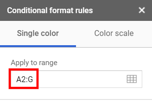
Expanding the Selection
Now, we are going to expand the range used in the “Apply to range” box all the way to column G by entering A2:G into the Apply to range input box. Specifying the range using this syntax will start the range at A2 and expand it down to the end of the spreadsheet and to the right through column G.
Video explanation
Fixing the Formula
If you stop now, it doesn’t change anything. You would think the formatting would extend across the entire row, but it doesn’t. What you need to do is change the formula.
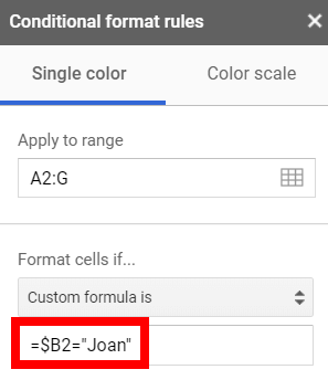
Before this change, the formula was incrementing one cell to right each time it calculated, just like any other spreadsheet formula when it is copied to another cell. Now, we have changed the formula from =B1="Joan" to =$B1="Joan". The dollar sign prevents the formula from moving to the right each time it decides if the conditional formatting criteria is being met. You have told your formula to continue looking at the same column for the criteria as it formats each cell. Just like you would if you were inside a spreadsheet cell, you used a dollar sign to indicate that value shouldn’t move when the formula moves.
The Entire Row is Highlighted
It’s working now since we fixed the column reference. Every row that was a sale by Joan has been highlighted.

I hope that was helpful. You can take this into your next presentation and wow everyone. You’ll just be amazing;) Have fun with it.
Jonathon says:
How would I highlight a row if a cell isn’t blank? I want to highlight an entire row if the cell in column F contains any text but not highlight it if the cell is blank.
Eric says:
Set a rule for exactly that. Usually you put down both the Good rule and the Bad rule. “IF F4 = anything, highlight” and “If F4 = blank, don’t highlight” (or use the default formatting in that case).
Skywokr says:
Using Google Sheets, Can cells with added notes be highlighted with conditional formatting? Say I want any cells with an added note to be highlighted orange…
Prolific Oaktree says:
I don’t know of a way to do that.
Mike says:
Is it possible to highlight multiple cells based off of the data in 1 cell, but instead of using single color, use a color scale?
Prolific Oaktree says:
No, the color scales don’t accept a custom formula. They work quite differently.
mauro says:
how highlight a row if a cell contiene a word…but not only that word?
Prolific Oaktree says:
Use the “Text contains” option in the Format rules.