There are no built-in options in Google Sheets that function on cells based on their formatting. There are a few crude methods to use functions by color, but these are not super-intuitive. Enter Power Tools.
How to Functions by Color in Power Tools
Power Tools is an add-on that gives our Google Sheets extra abilities, one of them being the ability to sum, average, et cetera, based on color, as explained in 📺this video.
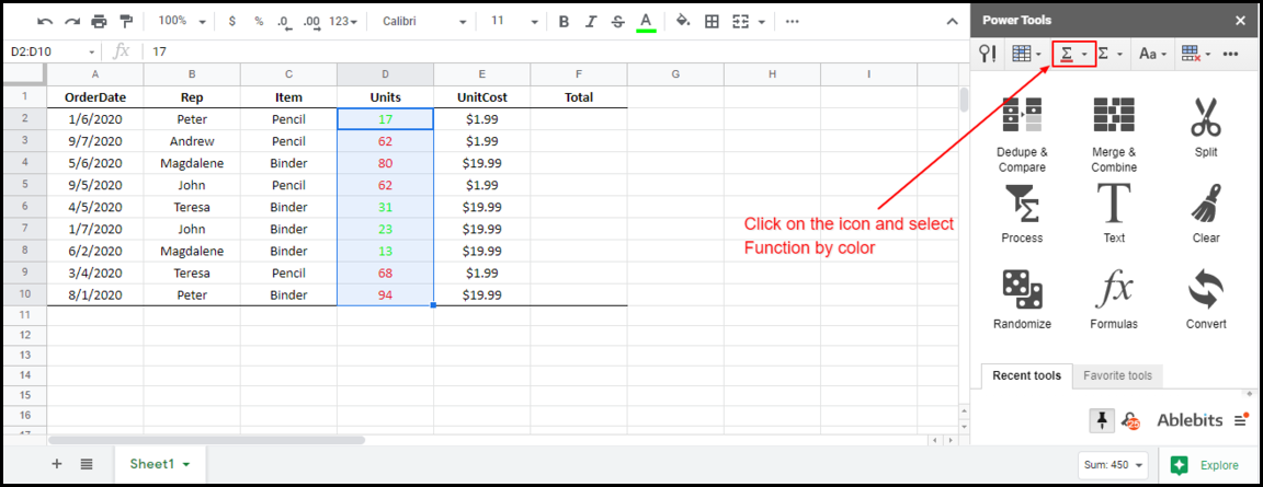
All units below 50 have a green font in the following dataset, while those above 50 have a red font (column D). How would we sum all the green values?

As mentioned, we need to use Power Tools.

After installing Power Tools, you can launch it via Add-ons > Power Tools > Start
After starting Power Tools, let’s find the total of all units that have a green font. First, we should highlight the range to which we want to apply a function. In our case, that’s D2:D10. Next, head over to the Power Tools sidebar, click on the red underlined summation icon, and select “Function by color”.

SUM by Color
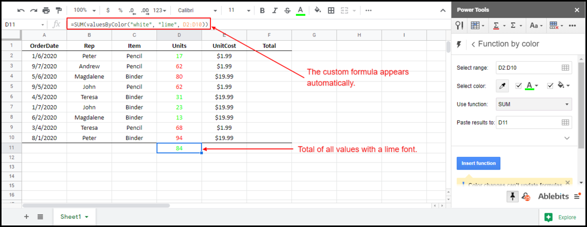
After clicking “Function by color”, we need to adjust the settings to match the formatting of the cells we want to work with. After changing the settings, we should set the background color to white and the font color to green (The actual name for the color is lime but, the most important thing is to make sure they are a visual match). There are quite a few functions we can apply to the selected range, but in our case, we’re interested in the SUM function.

Lastly, we click on “Insert function”. As a result of clicking on “Insert function”, a custom formula will appear on cell D11, and it computes the total of all values that have a lime font.
Notes on Power Tools

Things to note:
- The formula only recalculates if one of the values in the range changes. Therefore, any formatting changes will not trigger a recalculation until you modify one of the values.
- As aforementioned, you can apply other functions such as AVERAGE and PRODUCT.
0 thoughts on “How to use Functions by Color in Google Sheets”
Comments are closed.