-UPDATE- As of November 2016, their is a “Create a filter” option in the menus for Google Sheets on an iPad. You can find it by clicking the three vertically algined dots in the upper right hand corner of your spreadsheet. The tips below still apply to using the SORT function, but it not your only choice for sorting and filtering on an iPad now.

If you are looking for the SORT function in Google Sheets’ mobile app, good luck.  Much like the FILTER function in mobile Google Sheets, it has been relegated to the list of functions that must be typed in or found in the list of functions available in Sheets.  

Before you enter your SORT formula, you will want to select a cell in which to type it that will be the upper left most cell for the filtered list. This function write the data below and to the right of your starting point.  Once you find the right cell, enter the command using the following syntax:

=SORT(range, sort_column, is_ascending, [sort_column2, is_ascending2, ...])

In the formula above, SORT is the name of the function, range is the table of data that you want to be filtered, sort_column is the column by which you are sorting, and is_ascending is a true/false field to determine if you want the data sorted in ascending or decending order.  A value of TRUE for is_ascending would sort the data in ascending order (i.e. 1,2,3 or a,b,c).

Video explanation

Find more information on the SORT function at sheetshelp.com

One column

Let’s start with a simple example in the image below.

This is a small list of data. For whatever reason, you find the need to sort it.  Above is the data with the formula typed in a cell below it.  Below it the result after entering the formula. 

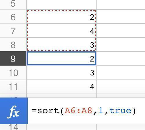
As you can see, the sort function creates a new list sorted by the parameters that you specified.  Be aware that the formula still remains in the cell in which you typed it. If you want to keep the data in this new list, you may want to consider copying it and pasting it as values. This will fix it in place even if the original data is changed.

Two columns

Next, let’s sort a table with two columns.  Select both rows, specify that you want to sort by the second row, and in decsending order..

=SORT(a15:b17,2,false)

This will create a new, sorted list.  Again, the filtered data is still dynamic.  If you change anything in the original list to be sorted, the new sorted list will also change.

Three columns

You can also specify a second column by which to sort data and a secondary level of orgainizing data.  The picture below is showing an easy example of this.

The output of this formula is as follows.  You can see that it sorted first by type of animal then by the number in the first column.

Conclusion

Having the sort function available, even if it is not in the menus, can be quite handy when you are working on a mobile device.  For larger sets of data, the sort function can be faster and more accurate than sorting data manually.  Enjoy and happy spreadsheeting to you all.