There are no built-in options in Google Sheets that function on cells based on their formatting. There are a few crude methods to use functions by color, but these are not super-intuitive. Enter Power Tools.
How to Functions by Color in Power Tools
Power Tools is an add-on that gives our Google Sheets extra abilities, one of them being the ability to sum, average, et cetera, based on color, as explained in 📺this video.
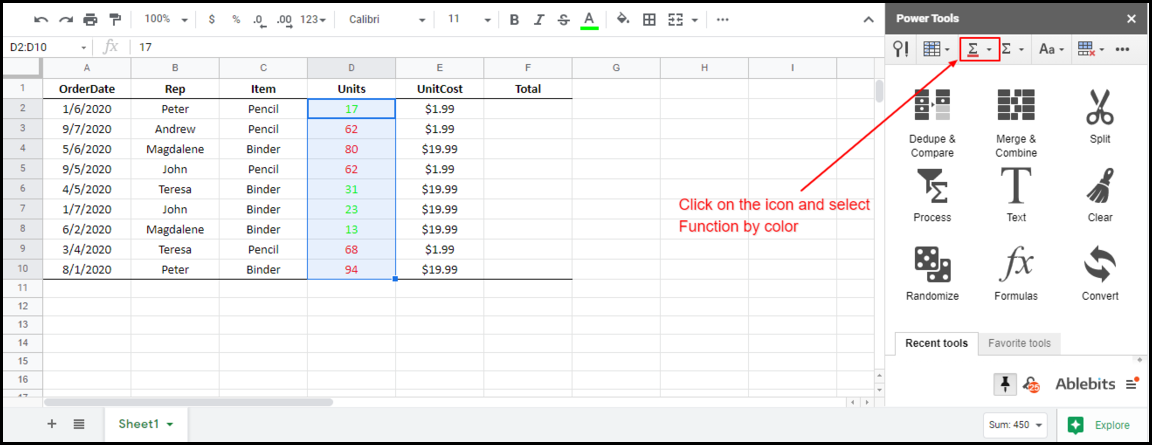
All units below 50 have a green font in the following dataset, while those above 50 have a red font (column D). How would we sum all the green values?
After installing Power Tools, you can launch it via Add-ons > Power Tools > Start
After starting Power Tools, let’s find the total of all units that have a green font. First, we should highlight the range to which we want to apply a function. In our case, that’s D2:D10. Next, head over to the Power Tools sidebar, click on the red underlined summation icon, and select “Function by color”.
SUM by Color
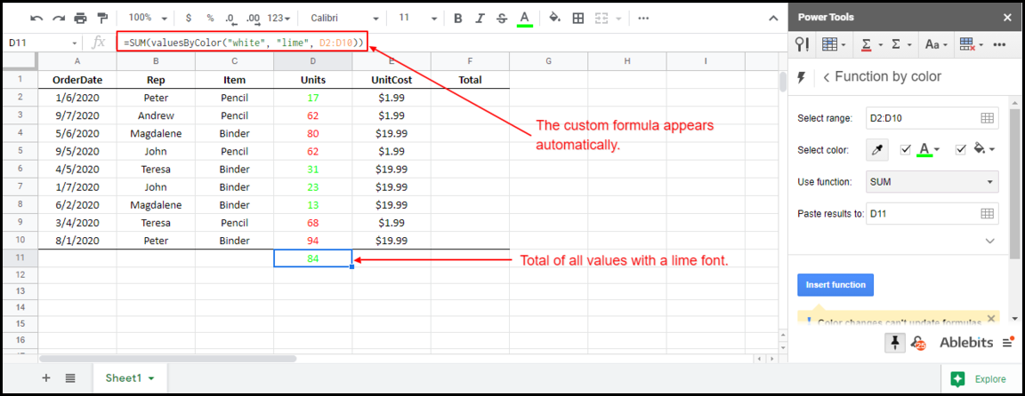
After clicking “Function by color”, we need to adjust the settings to match the formatting of the cells we want to work with. After changing the settings, we should set the background color to white and the font color to green (The actual name for the color is lime but, the most important thing is to make sure they are a visual match). There are quite a few functions we can apply to the selected range, but in our case, we’re interested in the SUM function.
Lastly, we click on “Insert function”. As a result of clicking on “Insert function”, a custom formula will appear on cell D11, and it computes the total of all values that have a lime font.
Notes on Power Tools
Things to note:
The formula only recalculates if one of the values in the range changes. Therefore, any formatting changes will not trigger a recalculation until you modify one of the values.
As aforementioned, you can apply other functions such as AVERAGE and PRODUCT.
Disclosure: This is an independently owned website that sometimes receives compensation from the company's mentioned products. Prolific Oaktree tests each product, and any opinions expressed here are our own.
You can have complete control over the look and feel of the numbers in your spreadsheet by using custom number formatting in Google Sheets. You can follow this example by starting with this template.
This article will walk you through the process of customizing the appearance of the numbers in your spreadsheet. Accordingly, it will teach you how to control your numbers’ visual presentation with currency signs, arrows, and more. Changing the look is called Custom Number Formatting. To have a comprehensive understanding of Custom Number Formatting, see this video from the Prolific Oaktree Youtube Channel.
Besides the default look, which presents your data in the black font color, you can infuse some level of creativity in your presentation by assigning different font colors to enhance the message of your presentation. For instance, you may want to present debits in red and credits in green.
Take a look at the image below.
Red and Green custom numbers
The data in red have a minus sign (-) before each, which indicates negative, hence, the use of red. On the other hand, the data in green is positive.
Changing the number formatting allows you to change the look, but the values of each cell will not change. It only gives it a different appearance through the color assigned to individual rows of data.
How To Custom Format Your Numbers in Google Sheets
The procedure is simple; locate your menu bar at the top of your spreadsheet and select Format>Number.
How to Format Numbers
After the number format menu appears, you will notice that there is a preset format for the display of your data. If that is what you want, you do not need to change anything. Just click on it, and you have your option activated.
However, if you want to give the data in each of the cells on your spreadsheet a custom look, you need to dig deeper. We will walk through how to get that done.
Customize the Look of Your Numbers in Google Sheets
The way your spreadsheet looks is up to you. Therefore, if you are not satisfied with the general format, this is how you can change it.
Highlight the columns with the numbers to be changed.
Click on Format on the menu bar.
Click on Number from the pop-down menu.
Check if there are pre-defined number formats for you to use (if not).
Click on More Formats.
Click on More Number Formats.
A dialogue box will pop up for you to choose the syntax:
Custom Number format
The syntaxes are below:
Input
0; -0; “-“; “not a number”
Output
Formats a positive number with 0
Formats a negative number with -0
Shows zero as a dash (“-“).
Shows a non-number as “not a number.” Anything in quotes in programming as a syntax remains as it is. The quotes signify that it is a string variable. The semicolon is to separate the columns.
If you intend to format a long number such as “$8,000,000,” you would use the “$#,##0.00” syntax. If you don’t intend to include the decimal points, enter “$#,##” and click the “Apply” option. Voila!
How To Insert Currency Before a Number in Google Sheets
To insert a currency sign before your number, the sign should precede the numbers in the syntax dialogue box such as we have below:
$* 0.00 – positive
$* – 0.00 – negative
The asterisk (*) gives space between the number and the currency sign. The two zeroes after the decimal force the display of tenths and hundredths.
How to Add Color to Custom Number Formatting
As earlier stated, you can give colors to your numbers for easy understanding.
To achieve customized color for your data, type the following syntax:
0[Green]; -0[Red]; ‘-‘[Black]
NOTE: The name of the color for each number format will come after each of the numbers in parentheses. Make sure you enclose the color for each cell in square brackets (Check the image below).
For the image below, the name for positive numbers is GREEN. Negative numbers are assigned RED. Zero will appear in BLACK.
Custom Color format
How to Insert Special Characters in Your Data in Google Sheets
Adding special characters to your presentation can make your Google Sheet easier to understand.