Google Sheets – SUM or COUNT Values If Cells Have Notes

Overview

If you’re using Google Sheets and you have a list of amounts that you want to sum or count based on whether or not there are notes in the cells, there’s no built-in function to do it. However, there are a relatively easy set of steps to make your own functions to get it done. You’ll be able to COUNT based on cell notes and you’ll be able to SUM as well. Previously, we’ve made custom functions to COUNT or SUM by background color.

This video will walk you through the same steps described below.

Custom formulas in action

COUNT or SUM by note
Cells being counted and summed by notes

SUM if there are notes

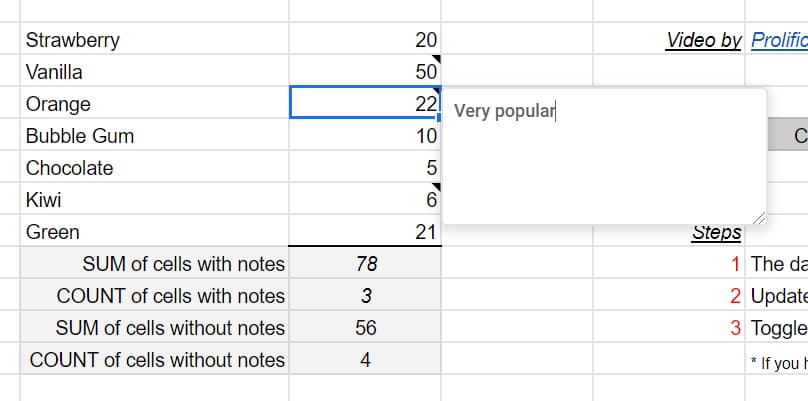
If you look in the live spreadsheet, you will see the custom formulas being used for summing based on whether a cell has notes. This does not work for comments, only notes. The summing is done by a formula with the nice little name of SumIfNote which takes the inputs of your range, TRUE/FALSE for with/without notes, and a trigger to recalculate as explained in the associated video.

formula for SumIfNote
Formula used to sum if there are notes

COUNT if there are notes

CountIfNote returns a 3 (which you can see above) since there are three cells with notes.

CountIfNote Formula
Formula to count cells if they contain notes
Watch the video

Creating custom formulas

It is far easier to grab a copy of the linked sheet. How do we make these functions and any other custom function that you’re so inclined to write? First, go to Tools and you go to Script editor.. and to copy and paste code below.

 /**
* @param {range} countRange Range to be evaluated
* @param {range} colorRef Cell with background color to be searched for in countRange
* @return {number}
* @customfunction
*/

function SumIfNote(sumRange, note, refresh) {
  var ss=SpreadsheetApp.getActive();
  var aSheet= ss.getActiveSheet();
  var sRange = aSheet.getRange(sumRange);
  var values = sRange.getValues();
  var sumResult=0;
  var rangeRow = sRange.getRow();
  var rangeColumn = sRange.getColumn();
  for(i=rangeRow; i<rangeRow+sRange.getNumRows(); i++) {
    for(j=rangeColumn; j<rangeColumn+sRange.getNumColumns(); j++) {
      if((aSheet.getRange(i, j, 1, 1).getNote() != "") == note) {
        sumResult += values[i-rangeRow][j-rangeColumn];
      }
    }
  }
  return sumResult;
}

function CountIfNote(sumRange, note, refresh) {
  var ss=SpreadsheetApp.getActive();
  var aSheet= ss.getActiveSheet();
  var sRange = aSheet.getRange(sumRange);
  var values = sRange.getValues();
  var countResult=0;
  var rangeRow = sRange.getRow();
  var rangeColumn = sRange.getColumn();
  for(i=rangeRow; i<rangeRow+sRange.getNumRows(); i++) {
    for(j=rangeColumn; j<rangeColumn+sRange.getNumColumns(); j++) {
      if((aSheet.getRange(i, j, 1, 1).getNote() != "") == note) {
        countResult += 1;
      }
    }
  }
  return countResult;
}

Script editor

After you go to Tools then Script editor, you come up with a blank screen. But if you don’t, do a new script file. Paste the code into the blank window. Repeat for each code section above and name them countColoredCells and sumColoredCells. For each file, the script editor puts the “.gs” at the end of the file name, indicating that it is a Google Script. After making these two, save them, return to your spreadsheet, and type in the formulas. It should work for you. See the video and linked sheet for further clarification.

 Live examples in Sheets

Go to the linked sheet for examples of counting cells by notes that you can study and use anywhere you would like.

Google Sheets – Count cells containing specific text

If you’re using Google Sheets and you want to count the occurrences of a certain letter or word, there’s a pretty easy function that you can use.

Looking for a word and only that word

In this first set of data in the image above and also in this linked spreadsheet, we will be counting any cells that contain the word “Yellow” and only that word. To count the occurrences of the word yellow in the range B2 to B9 you can use the count COUNTIF function as such: =COUNTIF(B2:B9,"yellow"). It performs a conditional count. In this case, only if the cell or ranges of cells is equal to Yellow. Yellow is not case-sensitive so this is going to pick up three instances even though B7 is not capitalized. If the COUNTIF technique is doing everything you need, then you’re done and there is no need to try anything more involved.

Looking for a word occurring anywhere a cell

COUNTIF with wildcard

Looking at this second set of data, things will get a little bit more complicated. We are looking for a certain word that occurs anywhere in any of these cells. First, you want to use COUNTIF again and give it a range =COUNTIF(C2:C9, "*Yellow*"). For this example, the range will be C2 to C9. If it has the word yellow and anything before which is what the asterisk means, and anything after it which is the second asterisk, then it should be counted. It just has to have yellow in some part of it. Anything can be nothing so it can start or end with yellow too. This function is also counting 3 because of the yellow plane, the yellow car, and the little yellow boat.

Case-Sensitivity

The COUNTIF function is not case-sensitive. To count cells with specific capitalization, follow the second example in this tutorial.

Using a plugin

As an alternative to the options above, you may want a plugin to do the heavy lifting for you. I like to use a plugin called Power Tools. This will give you a menu option with, among other things, advanced Find and Replace features. This will give you a list of all the occurrences of a word in your spreadsheet, but it won’t give you a count of them. Depending on the size of the spreadsheet, this may be the preferable option.

The Find and Replace Menu
Find and Replace Menu

I hope that was helpful and now you know the formula for counting any occurrences of any word that you’re looking for.

Β Live examples in Sheets

Go to this spreadsheet for examples counting specific text that you can study and use anywhere you would like.

Disclosure: This is an independently owned website that sometimes receives compensation from the company's mentioned products. Prolific Oaktree tests each product, and any opinions expressed here are our own.

COUNTA

Google Sheets – Count cells that are not blank

If you’re using Google sheets and you want to count the number of cells if they’re not blank, there are a couple different ways to do it and some complications that you might run into.

COUNTA usually works

I’m going to show you the easy way and a little bit harder way if you run into trouble. Let’s use COUNTA with the range from B3 to B9. The syntax, as also shown in the image above and the linked Google Sheet, is =COUNTA(B3:B9). This is the easy, straightforward way that’ll probably work most of the time. COUNTA is a built-in function. It will count any cell with a value and within the specified range. If that works for you, then you’re done. Don’t worry about it.

Video explanation

Longer formula
Longer formula

But, if we go to column C, things can get a little bit more complicated. This column looks like it has the same number of values, right? However, the COUNTA has the same range but is picking up seven instead of six. That’s happening because I snuck a blank space in C5. You may want to count this blank space since it is technically a value even though you cannot see it. If that’s the case, then then you’re done. COUNTA will work and the result is seven.

Longer function to not count white space

But, you may not want to count this blank cell. Accordingly, you may want to count what appears to have data in it, and you don’t really consider an empty space to be data. If this is the case, you have to use a more complicated formula. The function in cell C12, =SUMPRODUCT(--(LEN(C3:C9)>0)) is adding everything when the LEN function returns something greater than zero. LEN is counting the number of characters. The LEN function will not count the spaces that don’t really have any characters and, if that’s what you want, then that’s the way to get it done.

Now you have two different choices to count the number of cells that are not blank. A simple COUNTA for cells with no values at all, and the longer alternative, LEN, to exclude the empty spaces from the count.

 Live examples in Sheets

Go to this spreadsheet for examples of adding and subtracing days, months, or years that you can study and use anywhere you would like.
Column of numbers

Google Sheets – Count cells greater or less than an amount

If you’re using Google Sheets and you have a column of data in which you want to count the number of items that are greater or less than a certain amount, there are a couple of small nuances to it, but generally, it’s pretty easy.

Column of numbers
Column of numbers

Column of numbers with COUNT function
Numbers with a count

To perform this count using the data in the images above, we’ll be using the COUNTIF function in cell C11. This is a function that’s going to count a range if a certain criteria is met.

  • Place your cursor in cell C11 and type =COUNTIF(C3:C9,">30000"). The C3 is the start of the range and C9 is the end.
  • After you type the range into the function, enter a comma. That lets Google Sheets know that you are done with the range.
  • Then, enter the criteria surround by quotes. We’re going to do anything greater than 30,000. Don’t put a comma in your 30000 or it’s going to think it’s text instead of number.

After you entered the formula, you can see there are four items over 30,000 and this counted them. Easy as pie.

Video explanation


 Live examples in Sheets

Go tothis spreadsheet for examples of that you can study and use anywhere you would like.