Employee timesheet example

Create an Employee Timesheet Using Excel | Includes Overnight Shift

Are you using Microsoft Excel and you would like to record your employee’s working hours? Here’s a quick tutorial showing you how to do that, using Data Validation to make the process faster and easier.

You can use Excel as part of Office 365 or you can use the free online version. The free online version is good if you are a lighter user.

Here’s an example of a simple timesheet. This timesheet shows the date and time that employees have clocked in and clocked out, and shows the hours for each individual shift. It also shows the total hours for all the shifts.

Employee timesheet example

Data Validation for Date Entries

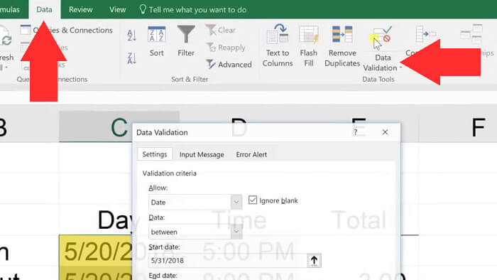
This sheet has been set up with data validation to make sure that the data entered for the dates and times are valid. Let’s take a look at that now. Highlight the column that has been used for the date entries, navigate to the Data ribbon, and left-click on Data Validation to bring up the window.

data validation

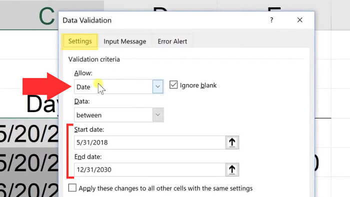
In the Data Validation window, you can set up rules for the cells in this column. Accordingly, we have only allowed date entries, and we have put in a range for the dates that are allowed to be entered in these cells. By allowing only date entries, if your user doesn’t enter a valid date, they’ll get an error alert prompting them to correct it. We’ll look at that in a moment.

data validation settings

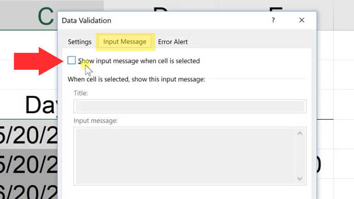
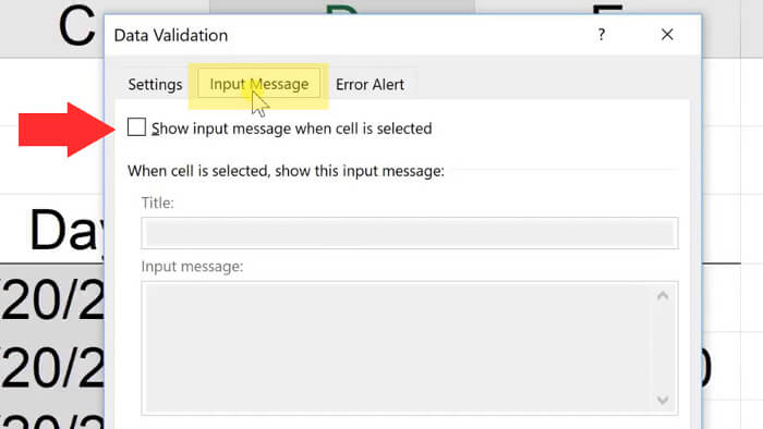
Next, click on the Input Message tab. After clicking, you will see that there’s a checkbox there to show input messages. This checkbox makes an input message pop up every time a user clicks on a cell to prompt them what to enter. However, after the first few times, this is probably going to be unnecessary. Therefore, we’ve unchecked that, but you can put a message there to prompt your user to enter a date.

input message

Error Alert Tab

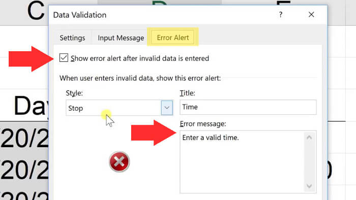
Click on the Error Alert tab. As you will see, we’ve checked the box to show an error alert when an invalid date is entered. As a result, the alert will show a message prompting your user to enter a valid date.

error alert

To test Data Validation for our date entries, we’ll go back to our spreadsheet and enter something that’s not a valid date to see what happens. For example, we’ll attempt to enter ‘June 1st, 2018’.

invalid date

Excel won’t like this because it doesn’t recognize the ‘st’, and we’ll get an error alert.

date error

To fix this, if you click ‘Retry’ and enter ‘6-1-18’, that’s fine and Excel will convert that to the correct format. Excel takes date entries in a variety of ways, but not every format will be recognised. Our error alert will make it clear when something is wrong.

Data Validation for Time Entries

We also have Data Validation for the time entries. To see this, highlight the time entry column and go to the Data ribbon. Left-click on Data Validation. Here, we’ve only allowed time entries, between midnight and midnight.

time data validation settings

Click on the Input Message tab. Again, we’ve unchecked this as we don’t need to see the prompt telling the user to enter a time value every single time an entry is made.

input message

Now click on the Error Alert tab. We’ve set it up here so that if the user doesn’t enter a valid time, it’s going to give an error alert prompting them to correct it.

validation error alert

In addition, to test the Data Validation for our time entries, we’ll enter an invalid time. We’ll try to enter ‘2pm’ which Excel doesn’t recognize as it wants a space between the ‘2’ and the ‘pm’.

invalid time

As a result of the bad entry, we get an error alert prompting us to enter a valid time.

invalid time error alert

Consequently, if we try again to enter ‘2 pm’ or ’14:00’ (military time), Excel will recognise it and turn it into the correct format. There are a number of ways we can make time entries in Excel. However, not every format will be recognised. Our error alert will let the user know when something an entry is invalid.

Using Formulas with Data Validation

As a result, we have data validation for all of the date and time entries. This is important, because we’ll be using formulas to calculate various values in the Total column.

Before we get into that, note that this timesheet can also do overnight shifts. If we put an example of that at the bottom, with the shift starting in the afternoon of the first day and ending in the morning of the second day, we’ll get the correct total in column E.

overnight shift

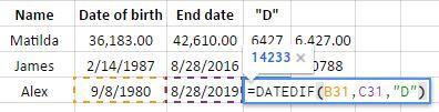
After that, let’s double-click on cell E9 and see what we’re using to calculate the number of hours for the shift.

formula

This is combining the date and time that the employee clocked out, and subtracting the combined date and time that they clocked in. This results in a fraction of a day for the length of the shift. Multiply by 24 to get the result in hours.

Next, to get the total for all the shifts, use a simple sum formula that sums all the hours for the shifts to get a total.

sum

That’s It!

In conclusion, with this simple timesheet, we can easily see how many hours we can pay our employee!

Using data validation, it’s easy to create a timesheet for your employees that alerts the user when they have entered invalid data. I hope this tutorial has been useful for you and your business!

Title of Sway

Embed a Live Excel Spreadsheet into a Microsoft Sway Presentation

If you’re using Microsoft’s Sway and you want to insert an Excel spreadsheet, there’s just a couple easy steps to do it.

Title of Sway
The title of your Sway

Create a new Sway and give it a title. I’ve called this one Embedding an Excel Spreadsheet.

Media group
Choose the media group

Next, click the plus sign to add more content. Choose the Media group then click the Embed option.

Embed
Choose the embed option

Video explanation

Create new Excel workbook
Create a new Excel workbook
Upload Excel workbook
Upload an existing Excel workbook

Sway is now waiting for the embed code. You need to get the code from Excel after you’ve uploaded it to OneDrive (or created it online to begin with). So, assuming you’ve uploaded your Excel flle, we’re going to step forward from that point. If you haven’t done that, you need to open up OneDrive and upload it.

Embed option in Excel
Embed option in Excel online

In the online Excel workbook, go to Share and embed and the code is ready at the bottom of the next window. You will be presented with a screen to select different parts of your spreadsheet, leave it at the default for now. Copy the embed code from your clipboard and go back to your Microsoft Sway. Go to the box waiting for your input, and paste the code.

Embed card with code
Sway card with embed code

You’ve embedded that Microsoft document. This is live. If you were to update this in Excel, this document that’s showing here would be updated. You can also interact with this document to a certain extent with the icon lower right hand corner. You can download it or print it.

Sway with embedded document
Columns for start date, end date, and name

Excel – Calculate age with the DATEDIF function

Calculating age in a spreadsheet can be a painful process using many of the formulas floating around the web today. Dates act strangely in spreadsheets so care must be taken when working with them. Fortunately, calculating age can be done much easier using a single function in Excel called DATEDIF. The DATEDIF function will return the difference between two dates in days, months, or years. Using these units in combination can get you a variety of output options.

Columns for start date, end date, and name
DATEDIF is not in the list of functions

This function is a carry over from the Lotus 1-2-3 days and is not an official function supported in Excel. Therefore, Excel won’t help you with hints when you type the function.

Google Sheets has this function in their core list of functions. There is no discussion of the MD error (see below) with Sheets.

Syntax

=DATEDIF(start_date,end_date,unit)

start_date Date at which to start the calculation

end_date Date at which to end the calculation

unit Type of output. Choices are “Y”,”M”,”D”,”YM”,”YD”, or “MD”.

  • Y – Number of whole years elapsed between start and end dates
    • YM – Number of months elapsed after the number of years shown with the “Y” unit. Will not exceed 11.
    • YD – Number of days elapsed after the number of years shown with the “Y” unit. No matter how many days after the last year, starts counting after end of last full year and is never over 364.
  • M – Number of whole months elapsed between start and end dates
    • MD – Number of days elapsed after the number of months shown with the “M” or “YM” unit. Can’t go higher than 30.
    • Beware that the MD option can cause errors.
  • D – Number of whole days elapsed between start and end dates


Video Explanation

Examples

Let’s say that you have three columns of data. As long as you have start and end dates, you are ready to go.

Columns for start date, end date, and name
Columns for name, start date, and end date

Now add 4 columns to the right for the DATEDIF formula with “Y”, “YM”, “YD”, and a column with them joined together. The Y, YM and MD are used as the “unit” in each respective column. The “Y” column is showing the person’s age in years. The “YM” is showing the number of months that have elapsed since the last year shown. The “MD” column is showing the number of days that have elapsed since the last whole month.

Columns with new formulas added
Y, YM, and MD units added

There are other types of units as well. This next example uses M and MD. Note that the number of months goes over twelve since the years are not in the formula’s output. The column using MD as the unit is the same calculation as above.

Columns with M and MD unites
M and MD units

This last example uses just the D unit. If you are just using this function to calculate days, it would be easier to just use a subtraction formula for the number of days. Dates in spreadsheets are actually stored as integers so they can easily be added and subtracted. The last column, which is unlabeled, contains a subtraction formula.

Column the D unit
Just days

If you want to calculate and age and have it always be current when you open the spreadsheet, consider using the function called TODAY as your end date. TODAY returns the current day.

insert ribbon

Text boxes in Excel – How and when to use them with Examples

Insert Text Box into Excel

If you are having trouble fitting text into a particular cell, or if you want a cleaner, easier method to show larger pieces of text, inserting a text box into your spreadsheet is a good solution.  In our post about using text boxes in spreadsheets, we see how many steps there are to inserting text if you do not use a text box.  The steps for inserting text using a text box are simple.

Click on the Insert Ribbon

insert ribbon 

and then click on Text Box.

insert text box

In the editing window, click where you want the upper left hand corner of the box.  While holding down the left button, drag down and to the right until the box is the size and shape you would like.  You are now ready to type as the cursor is already in the box waiting for you.

You can style the text by right clicking on the text the same way in which you would format other text.  In order to make the text box stand out, you can also right-click on the border of the box to change the weight of the border, the color, and the fill of the background.

style text box 2

Disclosure: This is an independently owned website that sometimes receives compensation from the company's mentioned products. Prolific Oaktree tests each product, and any opinions expressed here are our own.

overlapped text

Using text boxes in spreadsheets – Better than typing into a cell

Why use a text box?

Alternative to merging cells and wrapping text when using spreadsheets

Text boxes are used for large blocks of text in a spreadsheet.  One of the limitations of a spreadsheet is the clunkiness of inserting large pieces of text without interrupting the visual flow of the data.  The quickest way to insert text is to just type directly into a cell.  However, this presents several problems.

  • Too big for a cell

    • Inevitably, if you are typing more than a word or two, the content will flow out of the cell.  Visually, it will overlap the cell(s) to the right but the data won’t actually be in those other cells.  Because of this, if you add something into the cell that it is overlapping, the new content will appear over the text that you originally typed.

overlapped text

Merge cells

    • To work around this problem, one method is to merge the cells in which you want to display the text.

merged cells

  • Now the text in yellow resides in only one cell.  This can be helpful since there is no longer a chance that data will overlap it. However, you lose the option of using the cell to the right.  This can break the flow of the spreadsheet if you needed that cell. For longer strings of data, you can merge columns and rows of cells.

Text longer than two cells

merged cells but still too long


  • In the image above, an even longer piece of text has been inserted. This one overlaps more than one cell. We are back to the same problem.

merged cells columns and rows


After merging rows and columns

  • As you can see in the images above, when you merge a cell into different cells that live in different columns and rows, spreadsheets think that you still want the data to extend outside of the cell even if there is room inside of it.

  • Next, you have to apply wrap text

merged cells after wrap text


Wrap text applied to the cell

  •  What a pain!  As you can see, this are way too many steps for such a simple outcome.  Even worse, if you add lines of text to the cell, you will have to merge it again with neighboring cells.  Stop the insanity!!!


Text boxes save the day