While you may spend a lot of time combining data in Google Sheets, you may also need to split the data into different sheets. In Google Sheets, it’s possible to split rows of data into various sheets based on specified criteria. For instance, we could separate the following list of companies based on their headquarters. As seen in 📺this video, there is more than one way to achieve our intended end result.
Splitting rows in Google Sheets with the FILTER function
Let’s start by creating a list of companies headquartered in Australia.
Create a new sheet and name it “Australia”.
Copy the header row from Sheet 1 and paste it to the new sheet.
Next, we’re going to use the FILTER function to give us a list of only Australian-based companies. The syntax we should follow is =FILTER(range, criteria). For us, we want to return all the values in the range Sheet1!A2:C18, provided this criterion is met: column C is equal to Australia. Therefore our formula would be: =FILTER(Sheet1!A2:C18,Sheet1!C2:C18=“Australia”)
If we plug this formula into cell A2 of the sheet, Australia, we get the following output:
We successfully split rows of data in Google Sheets! The cells containing the word Australia are now in a separate sheet, but what if we were listing all companies worldwide? Would we have to manually create over 200 sheets and tweak the FILTER function accordingly? No we wouldn’t because there’s a powerful tool (excuse the pun 🙂 ) known as Power Tools that can do the heavy-lifting for us.
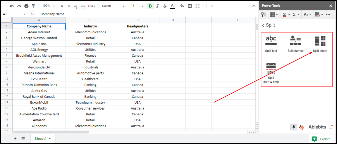
Once Power Tools is installed for the first time, a sidebar should appear on the right side of your sheet. If the sidebar doesn’t appear automatically, you can launch it via Add-ons > Power Tools > Start. After that, make sure you’re on Sheet1 and click on SPLIT in the Power Tools sidebar.
Upon clicking, a set of options should appear, giving us various choices of how we want to split the data. In our case, we want to split an entire sheet so that’s what we’re going to select.
Now the only thing that’s left is to specify the criteria by which we wish to split our data and the destination of the split sheets.
We get this as the output once we click on “Split”:
The entries have been separated into 3 tabs automatically. If we had 20 or 50 tabs, that’s the number of tabs that would appear.
Disclosure: This is an independently owned website that sometimes receives compensation from the company's mentioned products. Prolific Oaktree tests each product, and any opinions expressed here are our own.
This post is written to accompany the YouTube video showing how to combine multiple tables of data in your Google Sheet without using the QUERY function.
Oftentimes, data that you want to analyze is spread across multiple sheets and multiple files. If you want to combine tables found on multiple worksheets and/or multiple worksheets, these four different techniques will help you join them together. Each technique results in different output. Choose the one that works best for you.
These methods are meant for data with like headers and data types.
Using UNIQUE
Four circumstances covered
Keep Original Order
Keep the order of the original data by stacking each list.
Sorted
Sort the resultant table by any column.
Duplicates removed
Remove any duplicate lines of data if you don’t want them in your sample.
No blank rows
Remove any blank rows from your new table.
Also, data from another file can be pulled into these formulas using the IMPORTRANGE function.
To sort your spreadsheet data in a powerful and organized way, we can add Pivot Tables to isolate specific data, then Slicers to further sort those tables. These filters can sort data in a different way than the built-in pivot table filters and provide additional options for your data sets.
For this example, we will keep the source sheet as is and display the filtered list. The starting data is a typical spreadsheet we will utilize in two pivot tables.
To create the first Pivot Table, go to Data, then Pivot Table.
We will use the source as the entire table, including
headers. We will show the sales by item and an additional Pivot Table to
sort by item and date. Use the OmniPivot add-on to use more than one Data range.
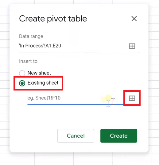
Select “Existing Sheet” and drop the table into G2 by
clicking the box to the right, then selecting G2.
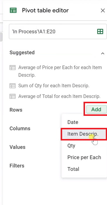
We’ll sort this by the sales quantity by item
description. Next to Rows in the Pivot Table Editor, click Add, and select Item
Description.
The Value will be “Quantity Sold.” We want this to be summed, so we will leave
this drop-down with the SUM value. This creates a simple table that sums the
sales by item description.
Create Another Pivot Table
To create the second Pivot Table, once again select Data then Pivot Table. We’ll use this table as a source and put this in G13. We’ll leave space because pivot tables expand and contract depending on what you do with them.
Second pivot table
First, we’ll add a row for the dates using the same method above, then right-click and group the dates. Go to “Create Pivot Date Group” and click “Month” for this example. We’ll do quantity again as the Value to populate the total sales for the items.
Date Group
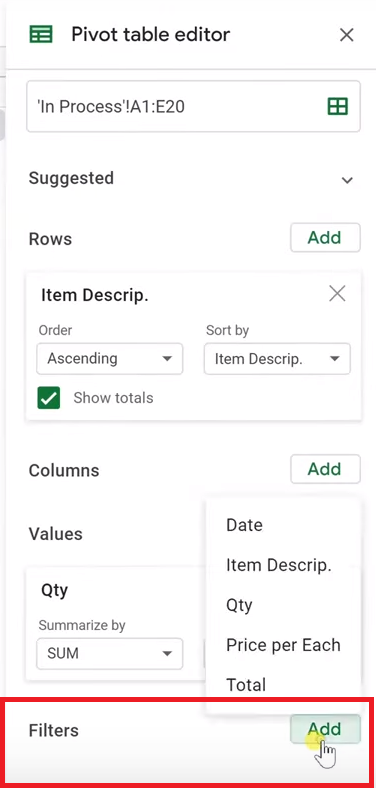
This means we’ll need to add items to this second Pivot
Table, so we’ll drop in another row by clicking the Add button next to Row, and
selecting Item Description.
These two different tables are showing the same data in
different ways – one by item description and one by item description and date.
Filter – First Method
The first way to filter these Pivot Tables is to create normal filters that will act on both of these pivot tables as long as they are in the same sheet and working on the same data. Left-click on the Pivot Table, then go to the bottom of the editor to add a filter – let’s say to filter Item Description.
If you left-click on the status, you can either filter by condition or by values (which will be the same in the slicer). We’re going to take “garden hose” out.
Filters are specific to one pivot table. You won’t see this
being filtered unless you look at the options in the editor. If we remove the filter, Garden Hoses will
come back to the table. This means that no one will be able to see that this
data is being filtered unless they look at the editor. This also only applies
to one Pivot Table.
New Filter Option – Slicers
Instead of filters, we’re going to use Slicers and see how they operate differently. Go to Data then Slicer.
Now it’s asking for the data range. Click the original
table, not the pivot table, for the data range. We’re going to slice the source
data.
Drag the slicer over to the right. Since we’ve already selected the range, it automatically populates in the Slicer options. We’re going to skip the column for now, and we’re going to make sure that the checkbox is selected so that it applies to Pivot Tables.
In addition, you can further customize the slicer by
choosing different colors, fonts, etc. Let’s leave it the way it is.
Let’s filter by item description. We can only do one column
right now – if we need more, we’ll need to make additional Slicers.
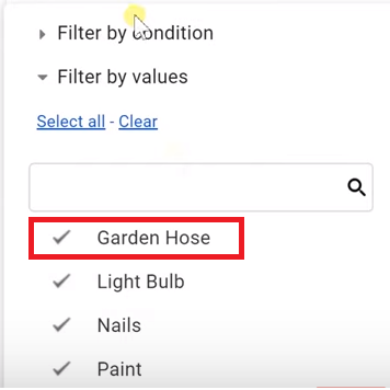
The first thing we’re going to notice is that the Slicer is
already here for everyone to see. There are the same options to filter by
conditions and values when you click it. We’re going to do the same thing again
and filter out Garden Hose. Start by clicking the Filter icon on the left.
Add Another Slicer
The data still exists but is hidden. If we want to filter by
date, we will have to add an additional Slicer. All the Slicers on one sheet
have to work with the same ranges. Additionally, they are sheet specific, so
they will only filter the data on the original sheet.
The changes we have been making will only work in our user
profile with our sheet, so if you want these settings to apply to additional
users, you need to edit the slicer and pick “Set Current Filters as
Default” – that way they will see the same filters that you have.
Let’s continue filtering by date. We’re going to select date once again, and “Filter by Condition.” We only want it if it’s after August 1st, 2019. This table only has July values on it.
Before I click “okay” we can see that this table
has July values in it. When we update it, it will only have august.
In this example, we will be looking at four different methods for sorting a table of data in Google Sheets. All of the examples are from this Google Sheet. We will review simple sorting, filter creation, utilizing the SMALL and LARGE functions, and using the SORTN function. These techniques can also be found in this this video on the Prolific Oaktree YouTube channel.
Sorting Data
The first technique is simply to sort the data in a sheet utilizing the menu options, then deleting what information we don’t want. This is a very rudimentary and simple method, but it unfortunately ends with us losing data (that we might need later).
First, begin by selecting the data that you want to sort, then go to “Data” in the top menu, and navigate to “Sort Range.” We specifically want to sort row C.
Click the “Data has a header row” box, and click the dropdown menu to “Run Time.”
Now that the data is sorted, you can manipulate it as you see fit, including deleting or moving the data you do not need. This technique, however, puts the data out of order and makes you lose the rest of the data.
Creating Filters
The second method of manipulating data is to select the data again, go to the Data menu again, and this time, instead of choosing sort, we will create a filter.
Filters can sort but have much more functionality. For this example, we will sort by Throw Distance to get the top three throwers. Click the dropdown at the right side of the header.
This dropdown organizes the data for you. You can sort it in various ways.
Hit Clear and then choose the longest three by scrolling down to the end and putting checkmarks on the last three values.
You can use functions in this menu for additional sorting capabilities. For this example, we will simply use the final three pieces of data. Since there are ties, the sorter decides to show all of these entries as well. The final sorted list is still in its original order.
The advantage of using Filters is that the data still exists and is still able to be interacted with. This means you won’t have to worry about missing data.
The LARGE and SMALL functions
The following two methods are much more powerful ways to manipulate and view your data that draw from the data without directly affecting it. We have created another area of the sheet where we can manipulate the data separately from the original list itself. Here, we will go over the LARGE and SMALL functions within Google Sheets.
What the LARGE function does is return the largest number in a chosen dataset. In this picture, we can see “$D$3:$D$21” which tells the function to look at the data collected from D3 through D21.
From here, we tell the function how to rank the data it finds. We can simply type in “1” or any other number depending on our needs, but in this case, we will refer to “H3,” which is the cell that contains our ‘Rank 1’.
We did this as a cell reference to H3 so I could drag the LARGE function down to do 2, 3, and 4.
Using ‘$’ on the range function in the formula tells the function, “Don’t shift this range down when I drag this formula down.” It’s a fixed reference for a range.
Rank 2 has the same formula, but by dragging it down, it is now looking for the second-largest value, and so on.
The SMALL function is simply the opposite of the LARGE function, and in the example here, it is picking the fastest run time and sorts to the slowest run time.
These functions don’t interact with any other row but also don’t affect the dataset itself.
SORTN Function
Native to Google Sheets and not found in Excel, the SORTN function is a powerful function that you can utilize to maximally sort to your desired preferences.
Start by highlighting all the data in your Sheet. This function will auto-populate all the fields, but you only have to type it once. Every variable is broken up with commas.
The function asks of these options: how many do you want me to return? We’ll put six. In the upper left corner of the screen, we can manually input 6 with another comma.
After 6, it asks what we would like to do with ties. For now, let’s choose 0.
The next variable is the column we are going to look at. This number is the number of columns from the left where the data resides. If we want to sort by throw distance, for example, it is the third column from the left, so we will enter 3.
Then we will select FALSE for “how to sort”. Then we hit Enter.
We have now picked up the longest six throw distances and it picked up names and jersey numbers, while leaving all the original data. Additionally, any changes to the original data will get automatically populated in the new function’s list.
Every situation is different, but now you have four options to consider. Let’s hope you can find the one that’s best for you!
Live examples in Sheets
Go to this spreadsheet for examples of methods to find the top or bottom values that you can study and use anywhere you would like.