If you have an Android phone and you have Windows 10 on your computer, you can project your screen from your phone onto your computer’s screen with no extra apps no cables. These steps and the accompanying screen shots are from a Samsung Galaxy S6.
Smart View
First, take your finger and swipe down from the top of your phone. Swipe down again and you’ll see some of these built-in apps. Swipe to the right and what you’re looking for is Smart View. Press Smart View with your finger and it’s going to start projecting your phone.
Smart View
Now go back to your computer. Type the Windows key and then type connect into box where you cursor is waiting at the bottom of the Start menu. After you type a few letters, the Connect app will be selected. Press enter to start it.
Search for Connect
Connect app
The Connect app will search for your phone’s signal that is being projecting by Smart View. Your phone and your computer will look for each other and then connect. That’s all. Two steps and we’re already pretty much done. You’ve projected your Android phone screen on to a computer running Windows 10.
-UPDATE- As of November 2016, their is a “Create a filter” option in the menus for Google Sheets on an iPad. You can find it by clicking the three vertically algined dots in the upper right hand corner of your spreadsheet. The tips below still apply to using the FILTER function, but it is not your only choice for filtering on an iPad now.
Most spreadsheet users are used to performing all of their functions through the menus with the click of a mouse. However, today’s mobile versions of these programs offer very few options through their menus. The FILTER function, much like the SORT function function, is one of those options that lost its coveted menu spot and has been relegated to the list of functions that must be typed in or found in the list of every function available in Sheets.
Before you enter your filter formula, you will want to select a cell that will be the upper left most cell for the filtered list. This function writes the data below and to the right of your starting point. Once you find the right cell, enter the command using the following syntax:
=FILTER(range, condition1, [condition2, ...])
In the formula above, FILTER is the name of the function, range is the table of data that you want to be filtered, and the conditions are how you want it to be sorted.
Video explanation
Find more information on the FILTER function at Sheetshelp.com.
One column
Let’s start with a simple example in the image below. This is a small list of data. For whatever reason, you find the need to filter it. A list this small would be easier to just manipulate by deleting what you don’t want, but it is kept simple so the illustrations can get right to the point.
As you can see, the filter function creates a new list with just the data left that you specified. Be aware that the formula still remains in the cell in which you typed it. If you want to keep the data in this new list, you may want to consider copying it and pasting it as values. This will fix it in place even if the original data is changed.
Two columns
Next, let’s sort the table based on criteria that resides in neighboring cells. Select both rows and use the second field of the formula for the sort criteria of b1:b4=”b”.
=FILTER(al:b4,b1:b4="b")
This will create a new, filtered list with just the rows that contain the letter “b” in the second column. Again, the filtered data is still dynamic. If you change anything in the original list to be sorted, the new sorted list will also change.
Three columns
You can also filter a table based on multiple criteria. The picture below is showing an easy example of this. The formula works as an AND statement, meaning that both conditions need to be TRUE in order for the data to be output by the function.
The output of this formula is as follows. The function only kept the data that had a “b” in column B AND a 3 in column C.
Follow image below for the live Google Sheet with this data
Conclusion
Having the filter function available, even it is not in the menus, can be quite handy when you are working on a mobile device. For larger sets of data, the filter function can be faster and more accurate than sorting data manually. Enjoy and happy spreadsheeting to you all.
-UPDATE- As of November 2016, there is a “Create a filter” option in the menus for Google Sheets on an iPad. You can find it by clicking the three vertically aligned dots in the upper right-hand corner of your spreadsheet. The tips below still apply to using the SORT function, but it is not your only choice for sorting and filtering on an iPad now.
Good luck if you are looking for the SORT option in Google Sheets mobile app. Much like the FILTER function in mobile Google Sheets, it has been relegated to the list of functions that must be typed in or found in the list of functions available in Sheets.
Before you enter your SORT formula, you will want to select a cell that will be the upper leftmost cell for the filtered list. This function writes the data below and to the right of your starting point. Once you find the right cell, enter the command using the following syntax:
In the formula above, SORT is the name of the function, the range is the table of data that you want to be filtered, sort_column is the column by which you are sorting, and is_ascending is a true/false field to determine if you want the data sorted in ascending or descending order. A value of TRUE for is_ascending would sort the data in ascending order (i.e., 1,2,3 or a,b,c).
Video explanation
Find more information on the SORT function at sheetshelp.com
One column
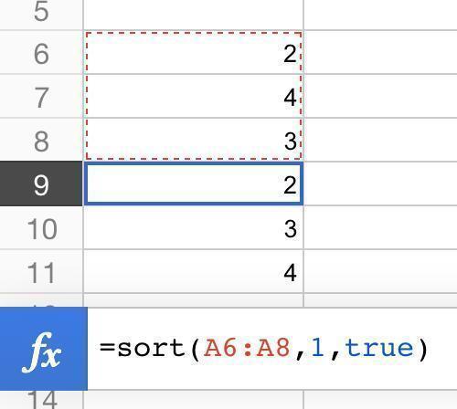
Let’s start with a simple example in the image below.
This is a small list of data. For whatever reason, you find the need to sort it. Above is the data with the formula typed in a cell below it. Below it the result after entering the formula.
As you can see, the sort function creates a new list sorted by the parameters that you specified. Be aware that the formula still remains in the cell in which you typed it. If you want to keep the data in this new list, you may want to consider copying it and pasting it as values. This will fix it in place even if the original data is changed.
Two columns
Next, let’s sort a table with two columns. Select both rows, specify that you want to sort by the second row, and in descending order..
=SORT(a15:b17,2,false)
This will create a new, sorted list. Again, the filtered data is still dynamic. If you change anything in the original list to be sorted, the new sorted list will also change.
Three columns
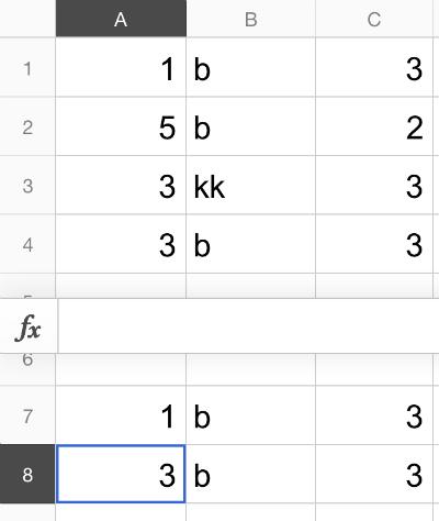
You can also specify a second column to sort data and a secondary level of organizing data. The picture below shows an easy example of this.
The output of this formula is as follows. You can see that it is sorted first by the type of animal and then by the number in the first column.
Conclusion
Having the sort function available, even if not in the menus, can be quite handy when working on a mobile device. The sort function can be faster and more accurate for larger data sets than manually sorting data. Enjoy and happy spreadsheeting to you all.
StaySorted Google Sheets Add-On
If you are sorting from the menus (instead of using the SORT function), you need to redo your sort every time you add a new row. That is unless you use the StaySorted add-on to automatically sort any new entries. Use it to help keep your spreadsheets organized.
There are several free options for online spreadsheet creating these days. The two most popular free options are Google’s Sheets and Apple’s Numbers, for which you need a free iCloud account. These programs can be used on a wide range of devices. Most of the screen shots below are from an iPad. Once you have chosen your program and created an account –
Start with a blank spreadsheet
Create a header row
Video explanation
Type the following values in cells A1 through A7.
Date – The date you made the deposit, wrote the check, etc. Note that this date does not always correspond to the date on which the transaction is posted to your bank account. This time lag creates the need to reconcile the account monthly. See how to do that in this post.
Check Number – This field is perhaps a bit outdated. 15 years ago, most payments coming out of a checking account would have been from paper checks. Presently, many are ACH’s or payments made directly from a bank’s website. However, this field can still be useful. You can use it simply for the checks that you still write, or you can be more creative with it and put confirmation numbers in it for online payments.
Cleared – This is the column that you use when you do your monthly reconciliation. You put an asterisk (or any other symbol) here when you see that the deposit or payment cleared the bank in the month in which you are performing your reconciliation.
Description – At the least, use this field to specify the payee for amounts going out and the payor for deposits coming in. Since it is a spreadsheet, and not a paper ledger, you can type as much as you want here. Take advantage of this. No one ever regrets having too much documentation. If you have a deposit from multiple people, write out all of their names and the amounts. Later, when you are trying to figure out if Mrs. So and So paid you, you can use search the spreadsheet (Ctl + F as a shortcut) and quickly find out.
Debit – Use this column for your payments out of the account. Admittedly, this is the opposite of what you would do if you were an accountant for a company using the double entry method. However, I chose to make my register this way because your bank calls payments debits and deposits credits so I find this less confusing.
Credit – Enter deposit amounts in this column
Balance – This will be the running total of your credits less your debits. Now, keeping this number large is your job!
Record your first entry
This is probably a deposit for an opening balance. The amount for this would go in the credit column. The formula for the Balance column is different on the first line. Note that formulas are started with the “=” sign. This is what tells a spreadsheet that your are entering a formula and it should display the result. The formula is simply:
=F2
This will display the value that you entered in the credit column. Note that the screenshots are from an iPad. Depending on what device you are using, the screen may look a bit different.
Use styles to display dollars and cents
As shown in the image above, numbers do not always display the way that you would like them to. When working with currency, it is typically helpful to see dollars and cents even when your amounts are in whole dollars. When you have a larger amount of transactions, having all of the number amounts display the same makes them easier to look through. If you don’t format these numbers, 1,000.01 will look significantly larger than 1000 when you are glancing at it. If they both display as 1,000.00 and 1,000.01, you will be able to tell the difference faster. Also, a comma can be helpful when the numbers get larger but a dollar sign can be redundant. If you are using Google Sheets, use the following steps to style the numbers.
First, select all of the columns to which you would like to apply the styles. If you only select certain cells, you will have to redo the styles when you add more rows.
Click on formatting and choose cell formatting then number format.
That should do it. Now your amounts will be easier to scan through.
Entering the next transaction
Now enter your next transaction in row 3. Whether this is a debit or a credit, this next formula will corrrectly capture it and add or subtract it from your balance. Note that the formula starts with an equals sign which is the universal technique for telling a spreadsheet that you are entering a formula instead of a value.
=G2-E3+E4
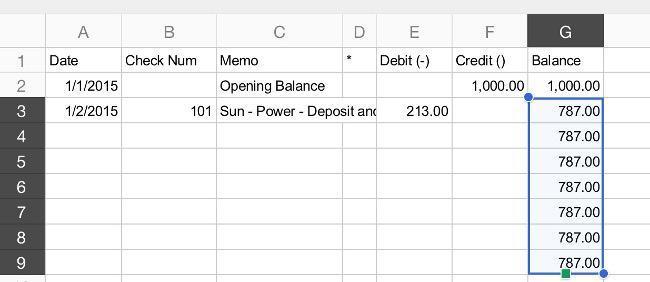
This formula is the only one that you will need from this point forward. You should copy this formula down this column for thirty lines or so, enough to give you some room to work without copying it again. Depending on what device you are using, there are multiple ways to copy a formula down. The most intuitive is copy and past the same way that you would with any other program. The easiest is to move the cursor to the lower right corner of the cell, until it changes to a different icon, then drag the outline down as far as you would like. When you copy formulas, the spreadsheet is smart enough to increment the cell references so they are always pointing at the appropriate line. If you are using Sheets on a tablet, select the rows you want to copy. Make sure you get a green dot on the rectangle that surrounds your selection as shown below. This image is shown after the green dot appeared and the user dragged it down with their finger.
When you are entering your descriptions, make them as long as you need to. You can search through your descriptions to find things later so pack them with the keywords that you think will be helpful. The next cell will just overlap the data but not erase it. See the highlighted portion below illustrating how the text is overlapped but is still saved and searchable.
See an example of this checkbook here as a shared Google Sheet. This spreadsheet is configured so that anyone can view it but not edit it.
Live examples in Sheets
Go to this spreadsheet for examples that you can study and use anywhere you would like.
You know have a simple, useful check register that you can access from anywhere that you have a web connection as Google Sheets and Apple Numbers can be used on mobile devices as well as laptops and desktops.


 Create a header row