In your Google Sheets workflow, it may sometimes be necessary to extract numbers from cells that contain a combination of both text and numbers. Perhaps you want to get the numbers to do further analysis, such as creating Pivot Tables. We can use various formulas for various unique situations. Let’s look at these formulas and a workaround that can save us a lot of time and effort.
Extracting numbers from text using the SPLIT function
The standard syntax for the SPLIT function is =SPLIT(text, delimiter). The delimiter tells the formula for how to separate the string. For instance, if we had a list of first names and second names separated by a comma, we can use the following formula to separate the names into separate cells: =SPLIT(text, ","). The comma is the delimiter in this case.

We can apply a similar concept to separate numbers that appear together with text in the same cell. How? By setting the delimiter to all characters that are not numbers. If we swap out the comma used in the previous example with the string, “qwertyuiopasdfghjklzxcvbnm, we are telling the formula to separate anything that isn’t in the domain of the mentioned string. Let’s see this in practice.

This only excluded letters of the alphabet from the output, and this is because the delimiter we specified only covers that scope. If we wanted brackets and colons excluded as well, we could add them to the delimiter. This separates the digits appearing before and after the character in question into different cells.
Extracting numbers from text using the REGEXREPLACE function
Another way we can extract numbers from a cell containing an assortment of numbers and text is using the REGEXREPLACE function. This function extracts all digits from a string and places them in one cell. The exact syntax used is =VALUE(REGEXREPLACE(text,"[^[:digit:]]",""))

One thing to note here is that REGEXREPLACE ignores any non-digit characters that appear between the numbers and merges the numbers in one cell. This returns the value of “0” if the text does not contain any numbers. If the string contains a pure number, the formula will return a VALUE error because it hasn’t found any non-digits to replace.
Using the REGEXEXTRACT function
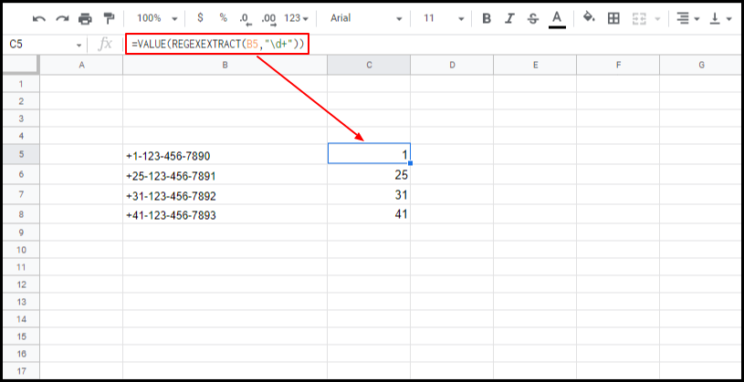
Instead of trying to extract all the numbers that occur within a string, we may be interested in just the first instance of digits that appear next to each other. For example, we could have a list of international telephone numbers that generally appear in the following format (+country dialing code)-(rest of the number. To extract the country prefix, we could use REGEXEXTRACT. The syntax would be =VALUE(REGEXEXTRACT(text,"\d+")).
These three ways to extract numbers from text are helpful in some ways, but they more or less are lacking in some capacity. In addition to that, if you’re not an avid spreadsheet user, things can get confusing and complicated for you at times. We can make things easier by using a Google Sheets add-on known as Power Tools.
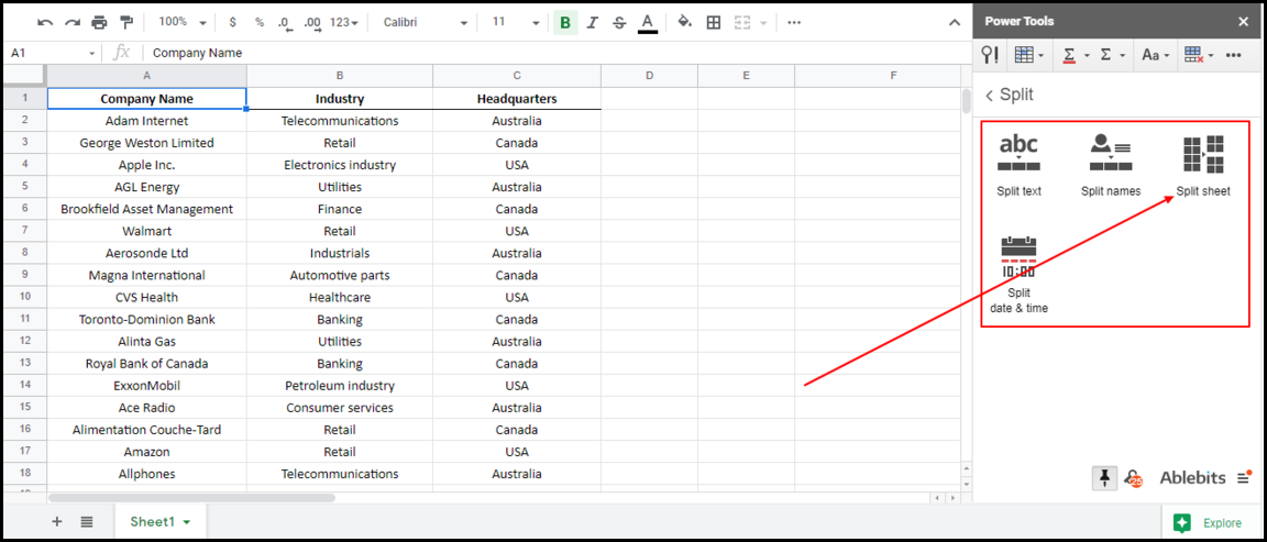
Extracting numbers from text using Power Tools add-on
Make sure to install Power tools before getting started. After installation, launch it via Add-ons > Power Tools.
On the sidebar that appears on the right, click on “Text” and then “Extract” and “Extract numbers”. Clicking on these options opens up an array of options for extracting numbers from our text.

What do the various options offer when extracting the numbers? Let’s explore them:
- If you specify that your numbers have decimal/thousand separators, the add-on will display all numbers, including those that appear after a comma and decimal point.
- If you check “Extract all occurrences”, this extracts all numbers regardless of their positions in the string. For example, the formula extracts 79 and 90 if a string is “79ogfgfh90”.
- There is an option to place occurrences in one cell or separate cells.
- You can choose to display results in a new column. By default, this displays the results to the right of the selected cells. This overwrites any data that exists in that column. However, if we select “Insert new column with results to the right”, it inserts new columns/columns with the extracted data.
- Finally, we can remove the extracted data from the source by selecting “Clear the extracted text from the source data”. This option could come in handy if we’re interested in the remaining text rather than the numbers extracted.