You may be looking for AutoSum in Google Sheets, but you won’t find it in the built-in menus.
AutoSum in Excel
Traditionally in Microsoft Excel, you would sum, multiply or divide values in a range by keying in the respective function and then specifying the range. You would add the total number of units In the following dataset by applying the formula, “=SUM(D2:D10)“.
However, as demonstrated in 📺this video, Excel provides a built-in intelligent function that automatically detects the range we wish to sum, known as AutoSum. If we place the cursor on cell D11 and click on AutoSum, Excel will figure out on its own that we intend to sum the range, D2:D10.
AutoSum in Google Sheets
Could we do the same in Google Sheets? Well, it’s not as impressive as in Excel. Instead of auto-detecting the range, Google Sheets merely inserts the specified function without the range.
We could solve this problem using a third-party add-on known as Power Tools.
After you install Power Tools, you can launch it via Add-ons > Power Tools > Start.
Now that we have the plugin installed, we can repeat the AutoSum operation we did in Excel. To achieve this, click on the cell that needs to add up the total. In our case, we want to get the Units total, so the cell is D11. Now that you have selected the units, head over to the sidebar and click on the AutoSum icon, Σ (not to be confused with the red-underlined Σ). Next, click on SUM in the drop-down that appears. After clicking, the total automatically appears in the cell we selected.
Things to note:
You can execute operations besides addition using the Power Tools add-on. The drop-down next to the icon provides a wide selection of functions to apply.
There’s an AutoSum by color function in Power Tools, which sums values based on background color and the text color. Find more on that here.
Disclosure: This is an independently owned website that sometimes receives compensation from the company's mentioned products. Prolific Oaktree tests each product, and any opinions expressed here are our own.
If you’re using Google Sheets and you have a list of amounts that you want to sum or count based on whether or not there are notes in the cells, there’s no built-in function to do it. However, there are a relatively easy set of steps to make your own functions to get it done. You’ll be able to COUNT based on cell notes and you’ll be able to SUM as well. Previously, we’ve made custom functions to COUNT or SUM by background color.
This video will walk you through the same steps described below.
Custom formulas in action
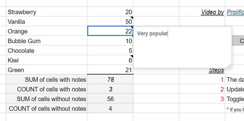
Cells being counted and summed by notes
SUM if there are notes
If you look in the live spreadsheet, you will see the custom formulas being used for summing based on whether a cell has notes. This does not work for comments, only notes. The summing is done by a formula with the nice little name of SumIfNote which takes the inputs of your range, TRUE/FALSE for with/without notes, and a trigger to recalculate as explained in the associated video.
Formula used to sum if there are notes
COUNT if there are notes
CountIfNote returns a 3 (which you can see above) since there are three cells with notes.
Formula to count cells if they contain notes
Watch the video
Creating custom formulas
It is far easier to grab a copy of the linked sheet. How do we make these functions and any other custom function that you’re so inclined to write? First, go to Tools and you go to Script editor.. and to copy and paste code below.
 /**
* @param {range} countRange Range to be evaluated
* @param {range} colorRef Cell with background color to be searched for in countRange
* @return {number}
* @customfunction
*/

function SumIfNote(sumRange, note, refresh) {
  var ss=SpreadsheetApp.getActive();
  var aSheet= ss.getActiveSheet();
  var sRange = aSheet.getRange(sumRange);
  var values = sRange.getValues();
  var sumResult=0;
  var rangeRow = sRange.getRow();
  var rangeColumn = sRange.getColumn();
  for(i=rangeRow; i<rangeRow+sRange.getNumRows(); i++) {
    for(j=rangeColumn; j<rangeColumn+sRange.getNumColumns(); j++) {
      if((aSheet.getRange(i, j, 1, 1).getNote() != "") == note) {
        sumResult += values[i-rangeRow][j-rangeColumn];
      }
    }
  }
  return sumResult;
}

function CountIfNote(sumRange, note, refresh) {
  var ss=SpreadsheetApp.getActive();
  var aSheet= ss.getActiveSheet();
  var sRange = aSheet.getRange(sumRange);
  var values = sRange.getValues();
  var countResult=0;
  var rangeRow = sRange.getRow();
  var rangeColumn = sRange.getColumn();
  for(i=rangeRow; i<rangeRow+sRange.getNumRows(); i++) {
    for(j=rangeColumn; j<rangeColumn+sRange.getNumColumns(); j++) {
      if((aSheet.getRange(i, j, 1, 1).getNote() != "") == note) {
        countResult += 1;
      }
    }
  }
  return countResult;
}
Script editor
After you go to Tools then Script editor, you come up with a blank screen. But if you don’t, do a new script file. Paste the code into the blank window. Repeat for each code section above and name them countColoredCells and sumColoredCells. For each file, the script editor puts the “.gs” at the end of the file name, indicating that it is a Google Script. After making these two, save them, return to your spreadsheet, and type in the formulas. It should work for you. See the video and linked sheet for further clarification.
Live examples in Sheets
Go to the linked sheet for examples of counting cells by notes that you can study and use anywhere you would like.
To sort your spreadsheet data in a powerful and organized way, we can add Pivot Tables to isolate specific data, then Slicers to further sort those tables. These filters can sort data in a different way than the built-in pivot table filters and provide additional options for your data sets.
For this example, we will keep the source sheet as is and display the filtered list. The starting data is a typical spreadsheet we will utilize in two pivot tables.
To create the first Pivot Table, go to Data, then Pivot Table.
We will use the source as the entire table, including
headers. We will show the sales by item and an additional Pivot Table to
sort by item and date. Use the OmniPivot add-on to use more than one Data range.
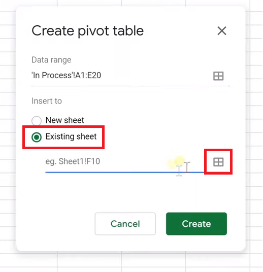
Select “Existing Sheet” and drop the table into G2 by
clicking the box to the right, then selecting G2.
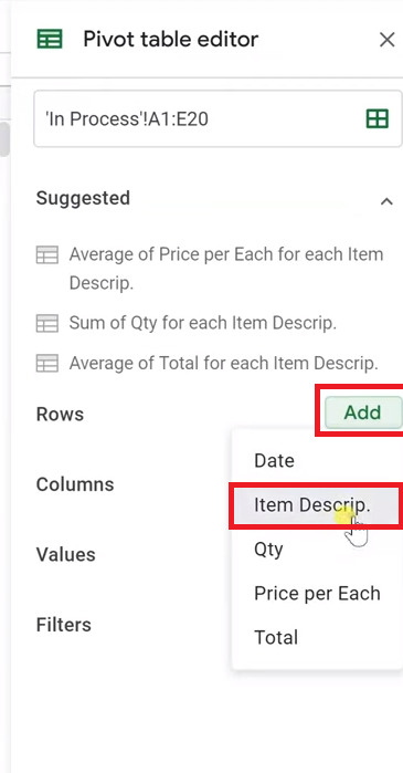
We’ll sort this by the sales quantity by item
description. Next to Rows in the Pivot Table Editor, click Add, and select Item
Description.
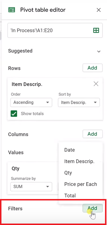
The Value will be “Quantity Sold.” We want this to be summed, so we will leave
this drop-down with the SUM value. This creates a simple table that sums the
sales by item description.
Create Another Pivot Table
To create the second Pivot Table, once again select Data then Pivot Table. We’ll use this table as a source and put this in G13. We’ll leave space because pivot tables expand and contract depending on what you do with them.
Second pivot table
First, we’ll add a row for the dates using the same method above, then right-click and group the dates. Go to “Create Pivot Date Group” and click “Month” for this example. We’ll do quantity again as the Value to populate the total sales for the items.
Date Group
This means we’ll need to add items to this second Pivot
Table, so we’ll drop in another row by clicking the Add button next to Row, and
selecting Item Description.
These two different tables are showing the same data in
different ways – one by item description and one by item description and date.
Filter – First Method
The first way to filter these Pivot Tables is to create normal filters that will act on both of these pivot tables as long as they are in the same sheet and working on the same data. Left-click on the Pivot Table, then go to the bottom of the editor to add a filter – let’s say to filter Item Description.
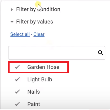
If you left-click on the status, you can either filter by condition or by values (which will be the same in the slicer). We’re going to take “garden hose” out.
Filters are specific to one pivot table. You won’t see this
being filtered unless you look at the options in the editor. If we remove the filter, Garden Hoses will
come back to the table. This means that no one will be able to see that this
data is being filtered unless they look at the editor. This also only applies
to one Pivot Table.
New Filter Option – Slicers
Instead of filters, we’re going to use Slicers and see how they operate differently. Go to Data then Slicer.
Now it’s asking for the data range. Click the original
table, not the pivot table, for the data range. We’re going to slice the source
data.
Drag the slicer over to the right. Since we’ve already selected the range, it automatically populates in the Slicer options. We’re going to skip the column for now, and we’re going to make sure that the checkbox is selected so that it applies to Pivot Tables.
In addition, you can further customize the slicer by
choosing different colors, fonts, etc. Let’s leave it the way it is.
Let’s filter by item description. We can only do one column
right now – if we need more, we’ll need to make additional Slicers.
The first thing we’re going to notice is that the Slicer is
already here for everyone to see. There are the same options to filter by
conditions and values when you click it. We’re going to do the same thing again
and filter out Garden Hose. Start by clicking the Filter icon on the left.
Add Another Slicer
The data still exists but is hidden. If we want to filter by
date, we will have to add an additional Slicer. All the Slicers on one sheet
have to work with the same ranges. Additionally, they are sheet specific, so
they will only filter the data on the original sheet.
The changes we have been making will only work in our user
profile with our sheet, so if you want these settings to apply to additional
users, you need to edit the slicer and pick “Set Current Filters as
Default” – that way they will see the same filters that you have.
Let’s continue filtering by date. We’re going to select date once again, and “Filter by Condition.” We only want it if it’s after August 1st, 2019. This table only has July values on it.
Before I click “okay” we can see that this table
has July values in it. When we update it, it will only have august.
In this example, we will be looking at four different methods for sorting a table of data in Google Sheets. All of the examples are from this Google Sheet. We will review simple sorting, filter creation, utilizing the SMALL and LARGE functions, and using the SORTN function. These techniques can also be found in this this video on the Prolific Oaktree YouTube channel.
Sorting Data
The first technique is simply to sort the data in a sheet utilizing the menu options, then deleting what information we don’t want. This is a very rudimentary and simple method, but it unfortunately ends with us losing data (that we might need later).
First, begin by selecting the data that you want to sort, then go to “Data” in the top menu, and navigate to “Sort Range.” We specifically want to sort row C.
Click the “Data has a header row” box, and click the dropdown menu to “Run Time.”
Now that the data is sorted, you can manipulate it as you see fit, including deleting or moving the data you do not need. This technique, however, puts the data out of order and makes you lose the rest of the data.
Creating Filters
The second method of manipulating data is to select the data again, go to the Data menu again, and this time, instead of choosing sort, we will create a filter.
Filters can sort but have much more functionality. For this example, we will sort by Throw Distance to get the top three throwers. Click the dropdown at the right side of the header.
This dropdown organizes the data for you. You can sort it in various ways.
Hit Clear and then choose the longest three by scrolling down to the end and putting checkmarks on the last three values.
You can use functions in this menu for additional sorting capabilities. For this example, we will simply use the final three pieces of data. Since there are ties, the sorter decides to show all of these entries as well. The final sorted list is still in its original order.
The advantage of using Filters is that the data still exists and is still able to be interacted with. This means you won’t have to worry about missing data.
The LARGE and SMALL functions
The following two methods are much more powerful ways to manipulate and view your data that draw from the data without directly affecting it. We have created another area of the sheet where we can manipulate the data separately from the original list itself. Here, we will go over the LARGE and SMALL functions within Google Sheets.
What the LARGE function does is return the largest number in a chosen dataset. In this picture, we can see “$D$3:$D$21” which tells the function to look at the data collected from D3 through D21.
From here, we tell the function how to rank the data it finds. We can simply type in “1” or any other number depending on our needs, but in this case, we will refer to “H3,” which is the cell that contains our ‘Rank 1’.
We did this as a cell reference to H3 so I could drag the LARGE function down to do 2, 3, and 4.
Using ‘$’ on the range function in the formula tells the function, “Don’t shift this range down when I drag this formula down.” It’s a fixed reference for a range.
Rank 2 has the same formula, but by dragging it down, it is now looking for the second-largest value, and so on.
The SMALL function is simply the opposite of the LARGE function, and in the example here, it is picking the fastest run time and sorts to the slowest run time.
These functions don’t interact with any other row but also don’t affect the dataset itself.
SORTN Function
Native to Google Sheets and not found in Excel, the SORTN function is a powerful function that you can utilize to maximally sort to your desired preferences.
Start by highlighting all the data in your Sheet. This function will auto-populate all the fields, but you only have to type it once. Every variable is broken up with commas.
The function asks of these options: how many do you want me to return? We’ll put six. In the upper left corner of the screen, we can manually input 6 with another comma.
After 6, it asks what we would like to do with ties. For now, let’s choose 0.
The next variable is the column we are going to look at. This number is the number of columns from the left where the data resides. If we want to sort by throw distance, for example, it is the third column from the left, so we will enter 3.
Then we will select FALSE for “how to sort”. Then we hit Enter.
We have now picked up the longest six throw distances and it picked up names and jersey numbers, while leaving all the original data. Additionally, any changes to the original data will get automatically populated in the new function’s list.
Every situation is different, but now you have four options to consider. Let’s hope you can find the one that’s best for you!
Live examples in Sheets
Go to this spreadsheet for examples of methods to find the top or bottom values that you can study and use anywhere you would like.
If you are using Google Slides to create a presentation with data from a Google Sheet, you may want to show that data as a linked table. If you create the table in Google Slides with no linking, it will not update if the data in the Google Sheet changes. Also, this is double work as the data is already in the Sheet, so re-typing it is a waste of time. Below are instructions on how to embed a live Google Sheet directly into your Google Slide. The table that is created will update with one-click and can be styled however you like. Live links to the Slide and Sheet shown in this tutorial are at the end of this article.
Delete the existing text box
Slides wants a blank area for the table. If you have a text box in your slide, delete it to make a nice, big open space.
Text box to be deleted
Watch the video
Create the Sheet
You need a spreadsheet created in Google Sheets with the table of data that you want to display in your Google Slide. In your spreadsheet, highlight the range that you want, right-click, and select Copy.
Table to be copied
Paste it into your Slide
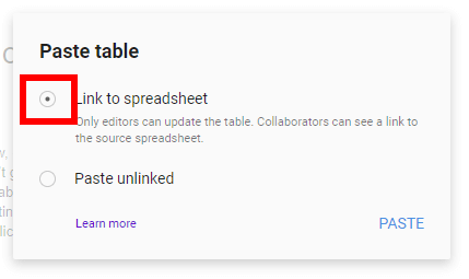
Then, go to the location in your Google Slides where you would like the table to be inserted. Right-click with your mouse and choose Paste. After clikcing, a window will pop-up asking you if you want to Link to spreadsheet or Paste unlinked. Choose Link to spreadsheet and click Paste.
Choose Link to spreadsheet
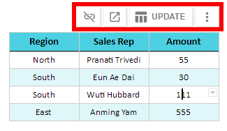
Oh yes, that’s a live, linked table that you’re seeing.
Google Slide with embedded Sheet
Working with your embedded table
Updating the embedded table
After linking the table, if you want to change the data within the table, you can go back to the Google Sheet to make the changes. When you come back to the Google Slide after making the changes, there will be a new option available to update the table when you right click on the table as shown in the picture below.
Adding rows
If you add rows to your table in Sheets, you may notice that the added rows don’t show up in the linked table in Slides. You will need to go back to the table in Slides after making the change, left click the more button (three vertical dots), and choose Change range.
Option to change the range
Conclusion
Following the steps above should provide you with an easy way to insert a live, linked spreadsheet into your Google Slides. Enjoy!