If you are using Google Sheets, you may be having some trouble finding how to insert a line. Once you have figured out how to insert it, getting it to be straight can be frustrating. Follow these easy steps to get it done.
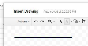
Go to Insert, then Drawing.
From here, choose Line.
Now, here’s where the real trick comes in. If you want to draw a line, go ahead. But, if you want to draw a straight line, hold down the shift key while you draw! There it is, a straight line.
If you are using Google Slides, you may be having some trouble finding how to insert a line. Once you have figured out how to insert it, getting it to be also straight can be frustrating. Follow these easy steps to get it done.
Go to menu bar and select line.
Line option on the main menu
Watch the video
Now, here’s where the real trick comes in. If you want to draw a line, go ahead. But, if you want to draw a straight line, hold down the shift key while you draw! There it is, a straight line.
-UPDATE- As of November 2016, their is a “Create a filter” option in the menus for Google Sheets on an iPad. You can find it by clicking the three vertically algined dots in the upper right hand corner of your spreadsheet. The tips below still apply to using the FILTER function, but it is not your only choice for filtering on an iPad now.
Most spreadsheet users are used to performing all of their functions through the menus with the click of a mouse. However, today’s mobile versions of these programs offer very few options through their menus. The FILTER function, much like the SORT function function, is one of those options that lost its coveted menu spot and has been relegated to the list of functions that must be typed in or found in the list of every function available in Sheets.
Before you enter your filter formula, you will want to select a cell that will be the upper left most cell for the filtered list. This function writes the data below and to the right of your starting point. Once you find the right cell, enter the command using the following syntax:
=FILTER(range, condition1, [condition2, ...])
In the formula above, FILTER is the name of the function, range is the table of data that you want to be filtered, and the conditions are how you want it to be sorted.
Video explanation
Find more information on the FILTER function at Sheetshelp.com.
One column
Let’s start with a simple example in the image below. This is a small list of data. For whatever reason, you find the need to filter it. A list this small would be easier to just manipulate by deleting what you don’t want, but it is kept simple so the illustrations can get right to the point.
As you can see, the filter function creates a new list with just the data left that you specified. Be aware that the formula still remains in the cell in which you typed it. If you want to keep the data in this new list, you may want to consider copying it and pasting it as values. This will fix it in place even if the original data is changed.
Two columns
Next, let’s sort the table based on criteria that resides in neighboring cells. Select both rows and use the second field of the formula for the sort criteria of b1:b4=”b”.
=FILTER(al:b4,b1:b4="b")
This will create a new, filtered list with just the rows that contain the letter “b” in the second column. Again, the filtered data is still dynamic. If you change anything in the original list to be sorted, the new sorted list will also change.
Three columns
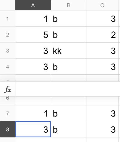
You can also filter a table based on multiple criteria. The picture below is showing an easy example of this. The formula works as an AND statement, meaning that both conditions need to be TRUE in order for the data to be output by the function.
The output of this formula is as follows. The function only kept the data that had a “b” in column B AND a 3 in column C.
Follow image below for the live Google Sheet with this data
Conclusion
Having the filter function available, even it is not in the menus, can be quite handy when you are working on a mobile device. For larger sets of data, the filter function can be faster and more accurate than sorting data manually. Enjoy and happy spreadsheeting to you all.
-UPDATE- As of November 2016, there is a “Create a filter” option in the menus for Google Sheets on an iPad. You can find it by clicking the three vertically aligned dots in the upper right-hand corner of your spreadsheet. The tips below still apply to using the SORT function, but it is not your only choice for sorting and filtering on an iPad now.
Good luck if you are looking for the SORT option in Google Sheets mobile app. Much like the FILTER function in mobile Google Sheets, it has been relegated to the list of functions that must be typed in or found in the list of functions available in Sheets.
Before you enter your SORT formula, you will want to select a cell that will be the upper leftmost cell for the filtered list. This function writes the data below and to the right of your starting point. Once you find the right cell, enter the command using the following syntax:
In the formula above, SORT is the name of the function, the range is the table of data that you want to be filtered, sort_column is the column by which you are sorting, and is_ascending is a true/false field to determine if you want the data sorted in ascending or descending order. A value of TRUE for is_ascending would sort the data in ascending order (i.e., 1,2,3 or a,b,c).
Video explanation
Find more information on the SORT function at sheetshelp.com
One column
Let’s start with a simple example in the image below.
This is a small list of data. For whatever reason, you find the need to sort it. Above is the data with the formula typed in a cell below it. Below it the result after entering the formula.
As you can see, the sort function creates a new list sorted by the parameters that you specified. Be aware that the formula still remains in the cell in which you typed it. If you want to keep the data in this new list, you may want to consider copying it and pasting it as values. This will fix it in place even if the original data is changed.
Two columns
Next, let’s sort a table with two columns. Select both rows, specify that you want to sort by the second row, and in descending order..
=SORT(a15:b17,2,false)
This will create a new, sorted list. Again, the filtered data is still dynamic. If you change anything in the original list to be sorted, the new sorted list will also change.
Three columns
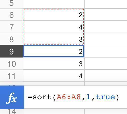
You can also specify a second column to sort data and a secondary level of organizing data. The picture below shows an easy example of this.
The output of this formula is as follows. You can see that it is sorted first by the type of animal and then by the number in the first column.
Conclusion
Having the sort function available, even if not in the menus, can be quite handy when working on a mobile device. The sort function can be faster and more accurate for larger data sets than manually sorting data. Enjoy and happy spreadsheeting to you all.
StaySorted Google Sheets Add-On
If you are sorting from the menus (instead of using the SORT function), you need to redo your sort every time you add a new row. That is unless you use the StaySorted add-on to automatically sort any new entries. Use it to help keep your spreadsheets organized.
Apple now offers its spreadsheet program to anyone that has an iCloud account. You can access it from most browsers which effectively opens up the program to Windows users. You do not get the same functionality that you would from iWork for Mac, but you can access the same files and perform the most common tasks.
Apple’s Numbers spreadsheet has a sharing option that allows you to invite others to collaborate with you on a spreadsheet. You can give them the ability to view or edit the spreadsheet and you can decide the level of privacy to afford it.
You can find this option by clicking on the sharing icon shown in the image above (the arrow inside the square). However, tread carefully, as this can leave your file open to viewing by others as will be explained in this article. At the time of the writing of this article, the sharing feature is only for the entire spreadsheet. There are no options to specify sharing and editing permissions on a specific cell, range, or worksheet. If you want to share only a portion of the spreadsheet, you will have to use another spreadsheet option such as Google’s Sheets which has more granular security features.
Video explanation
Once you choose to share the spreadsheet, you are presented with a few different options for how to share it. This is where things get a little fuzzy. If you are new to the concept of sharing documents over the web, it is important that you understand what is happening here.
Before you share anything, your files are locked down in iCloud and only someone who knows your username and password can access them. Hopefully that’s just you. However, if you choose to share a file, you are opening up this particular file to other users on the web outside of your iCloud account. Others will now be able to access the file even if they do not have an iCloud account.
Letting someone see but not edit
If you want to grant a user permission to see the spreadsheet, but not edit it, you choose this option during the sharing process.
However, there is a catch here. This spreadsheet is secured from others by the long, random URL that you see above for the spreadsheet link. This means that no one else will be able to stumble upon this spreadsheet because it is near impossible to guess the link. You should feel pretty comfortable that your spreadsheet is still private, but you should also understand what is making it private. If anyone found this URL, they would be able to see the spreadsheet. There is no login required for this option and no password has been specified. If you shared this spreadsheet with multiple people, then decided that one of the people should not be able to see it anymore, you cannot remove just that particular user’s access. If you still want it to be shared, you would have to add a password and control who gets the password.
Letting someone edit
If you want to grant a user permission to use the spreadsheet with the same permissions that you have, specify “Allow Editing” during the sharing process shown in the picture above. This will give anyone with the link the ability to edit the spreadsheet.
Password protect
This is Number’s method of allowing a user to share a spreadsheet while still keeping it confidential. While other cloud spreadsheet programs allow you to share spreadsheets with specific people, Numbers gives you the ability only to share your password with specific people. This accomplishes the same thing but gets you there differently.
Conclusion
The options described above offer enough flexibility to allow simple collaboratoin in Numbers. As your spreadsheets get more complicated, you may encounter the needs to specify certain ranges or worksheets that you want to protect in different ways. If all you want to do is share spreadsheets with others to allow them to see or edit, then Numbers has the ability to get this done.