How to use Functions by Color in Google Sheets

There are no built-in options in Google Sheets that function on cells based on their formatting. There are a few crude methods to use functions by color, but these are not super-intuitive. Enter Power Tools.

How to Functions by Color in Power Tools

Power Tools is an add-on that gives our Google Sheets extra abilities, one of them being the ability to sum, average, et cetera, based on color, as explained in đź“şthis video.

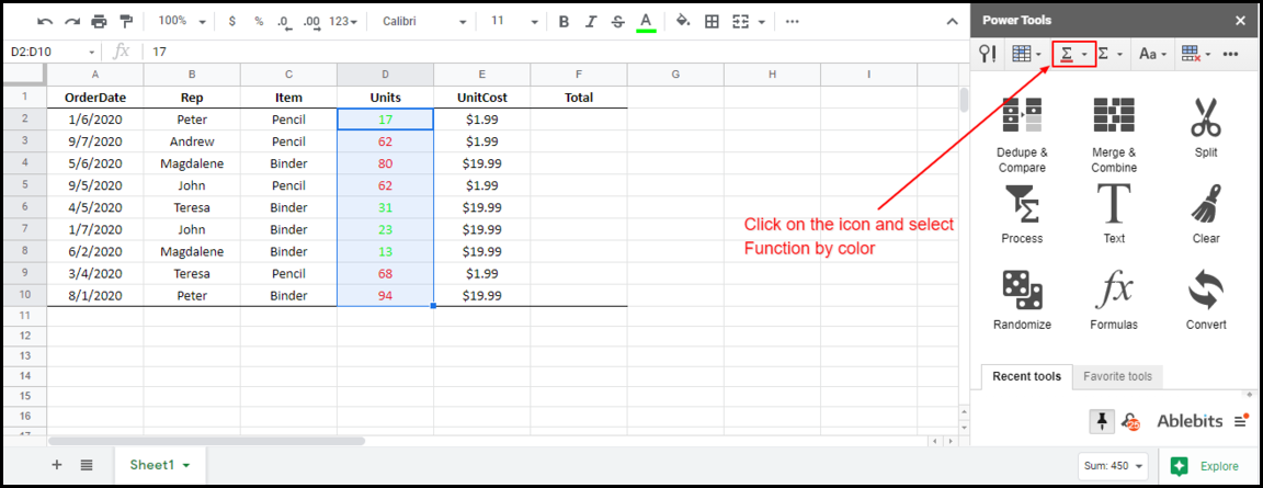
All units below 50 have a green font in the following dataset, while those above 50 have a red font (column D). How would we sum all the green values?
red and green font in your spreadsheet

As mentioned, we need to use Power Tools.

Power Tools menu showing to the right of the screen

After installing Power Tools, you can launch it via Add-ons > Power Tools > Start

After starting Power Tools, let’s find the total of all units that have a green font. First, we should highlight the range to which we want to apply a function. In our case, that’s D2:D10. Next, head over to the Power Tools sidebar, click on the red underlined summation icon, and select “Function by color”.

Icon to click to use functions by color

SUM by Color

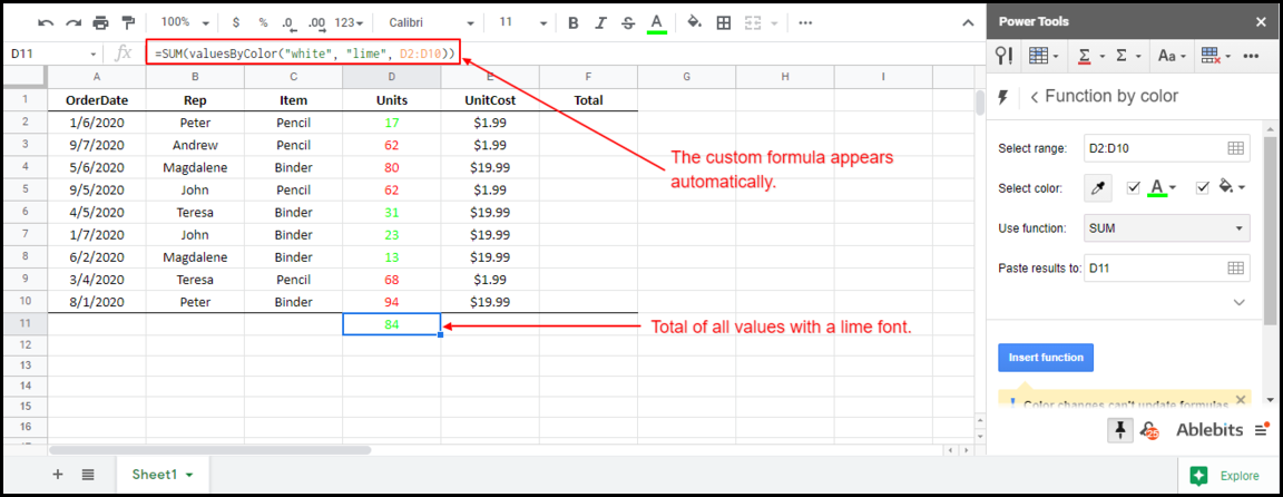
After clicking “Function by color”, we need to adjust the settings to match the formatting of the cells we want to work with. After changing the settings, we should set the background color to white and the font color to green (The actual name for the color is lime but, the most important thing is to make sure they are a visual match). There are quite a few functions we can apply to the selected range, but in our case, we’re interested in the SUM function.

parameters for using functions by color

Lastly, we click on “Insert function”. As a result of clicking on “Insert function”, a custom formula will appear on cell D11, and it computes the total of all values that have a lime font.

Notes on Power Tools

results of the function

Things to note:

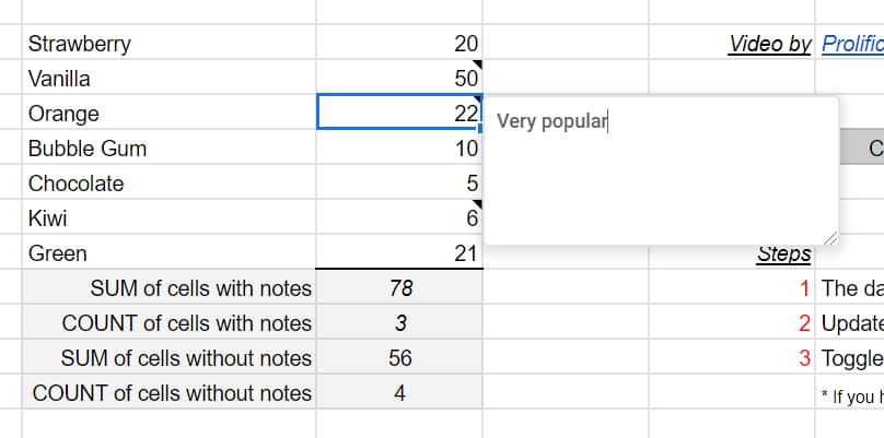
  • The formula only recalculates if one of the values in the range changes. Therefore, any formatting changes will not trigger a recalculation until you modify one of the values.
  • As aforementioned, you can apply other functions such as AVERAGE and PRODUCT.

Disclosure: This is an independently owned website that sometimes receives compensation from the company's mentioned products. Prolific Oaktree tests each product, and any opinions expressed here are our own.

AutoSum Function in Google Sheets

You may be looking for AutoSum in Google Sheets, but you won’t find it in the built-in menus.

AutoSum in Excel

Traditionally in Microsoft Excel, you would sum, multiply or divide values in a range by keying in the respective function and then specifying the range. You would add the total number of units In the following dataset by applying the formula, “=SUM(D2:D10)“.

column being SUMMED in Excel

However, as demonstrated in đź“şthis video, Excel provides a built-in intelligent function that automatically detects the range we wish to sum, known as AutoSum. If we place the cursor on cell D11 and click on AutoSum, Excel will figure out on its own that we intend to sum the range, D2:D10.

column of numbers being highlighted with autosum


AutoSum in Google Sheets

Could we do the same in Google Sheets? Well, it’s not as impressive as in Excel. Instead of auto-detecting the range, Google Sheets merely inserts the specified function without the range.

the SUM function appearing in Google Sheets

We could solve this problem using a third-party add-on known as Power Tools.


AutoSum in Google Sheets using Power Tools

To install Power Tools, click on this link.

After you install Power Tools, you can launch it via Add-ons > Power Tools > Start.


function menu in Power Tools


Now that we have the plugin installed, we can repeat the AutoSum operation we did in Excel. To achieve this, click on the cell that needs to add up the total. In our case, we want to get the Units total, so the cell is D11. Now that you have selected the units, head over to the sidebar and click on the AutoSum icon, ÎŁ (not to be confused with the red-underlined ÎŁ). Next, click on SUM in the drop-down that appears. After clicking, the total automatically appears in the cell we selected.


the result of autosum in Google Sheets using Power Tools


Things to note:

  • You can execute operations besides addition using the Power Tools add-on. The drop-down next to the icon provides a wide selection of functions to apply.
  • There’s an AutoSum by color function in  Power Tools, which sums values based on background color and the text color. Find more on that here.

Disclosure: This is an independently owned website that sometimes receives compensation from the company's mentioned products. Prolific Oaktree tests each product, and any opinions expressed here are our own.

Google Sheets – SUM or COUNT Values If Cells Have Notes

Overview

If you’re using Google Sheets and you have a list of amounts that you want to sum or count based on whether or not there are notes in the cells, there’s no built-in function to do it. However, there are a relatively easy set of steps to make your own functions to get it done. You’ll be able to COUNT based on cell notes and you’ll be able to SUM as well. Previously, we’ve made custom functions to COUNT or SUM by background color.

This video will walk you through the same steps described below.

Custom formulas in action

COUNT or SUM by note
Cells being counted and summed by notes

SUM if there are notes

If you look in the live spreadsheet, you will see the custom formulas being used for summing based on whether a cell has notes. This does not work for comments, only notes. The summing is done by a formula with the nice little name of SumIfNote which takes the inputs of your range, TRUE/FALSE for with/without notes, and a trigger to recalculate as explained in the associated video.

formula for SumIfNote
Formula used to sum if there are notes

COUNT if there are notes

CountIfNote returns a 3 (which you can see above) since there are three cells with notes.

CountIfNote Formula
Formula to count cells if they contain notes
Watch the video

Creating custom formulas

It is far easier to grab a copy of the linked sheet. How do we make these functions and any other custom function that you’re so inclined to write? First, go to Tools and you go to Script editor.. and to copy and paste code below.

 /**
* @param {range} countRange Range to be evaluated
* @param {range} colorRef Cell with background color to be searched for in countRange
* @return {number}
* @customfunction
*/

function SumIfNote(sumRange, note, refresh) {
  var ss=SpreadsheetApp.getActive();
  var aSheet= ss.getActiveSheet();
  var sRange = aSheet.getRange(sumRange);
  var values = sRange.getValues();
  var sumResult=0;
  var rangeRow = sRange.getRow();
  var rangeColumn = sRange.getColumn();
  for(i=rangeRow; i<rangeRow+sRange.getNumRows(); i++) {
    for(j=rangeColumn; j<rangeColumn+sRange.getNumColumns(); j++) {
      if((aSheet.getRange(i, j, 1, 1).getNote() != "") == note) {
        sumResult += values[i-rangeRow][j-rangeColumn];
      }
    }
  }
  return sumResult;
}

function CountIfNote(sumRange, note, refresh) {
  var ss=SpreadsheetApp.getActive();
  var aSheet= ss.getActiveSheet();
  var sRange = aSheet.getRange(sumRange);
  var values = sRange.getValues();
  var countResult=0;
  var rangeRow = sRange.getRow();
  var rangeColumn = sRange.getColumn();
  for(i=rangeRow; i<rangeRow+sRange.getNumRows(); i++) {
    for(j=rangeColumn; j<rangeColumn+sRange.getNumColumns(); j++) {
      if((aSheet.getRange(i, j, 1, 1).getNote() != "") == note) {
        countResult += 1;
      }
    }
  }
  return countResult;
}

Script editor

After you go to Tools then Script editor, you come up with a blank screen. But if you don’t, do a new script file. Paste the code into the blank window. Repeat for each code section above and name them countColoredCells and sumColoredCells. For each file, the script editor puts the “.gs” at the end of the file name, indicating that it is a Google Script. After making these two, save them, return to your spreadsheet, and type in the formulas. It should work for you. See the video and linked sheet for further clarification.

 Live examples in Sheets

Go to the linked sheet for examples of counting cells by notes that you can study and use anywhere you would like.