Start with a Pivot Table
If you have a table of data in Google Sheets and you want to look at it by a certain type of date, let’s say if you want to look at it by day of the week, the first thing that you want to do is create a Pivot Table. Using a Pivot Table will help you avoid constructing complex formulas with SUMIFS.
We are starting with a table, (shown in the image below) for our raw data and we will be creating the Pivot Table on a new sheet called Pivot Table 1 which is shown at the end of this article in the embedded view of the Sheet.
This tutorial assumes that you have already completed your Pivot Table and you have a basic knowledge of how to use it. See this video if you need some basic help on Pivot Tables.
If you need a primer on Pivot Tables, this video will walk you through them.
A well-formed table of data
As can be seen in the raw data above, it is important that you start with good data that has descriptive headers for each column and no empty rows. If you have empty rows, be sure to delete them before attempting to create a Pivot Table.
Once you are ready to create your Pivot Table, go to the menus, select Data then Pivot Table. The Blank Pivot table will be created on a new tab in your spreadsheet as shown in the picture below.

Add the Dates
To get the dates to be the first column on the left, we want dates to be the rows so add Ship Date to the Rows field. As mentioned above, working with pivot tables is a lot easier if you have descriptive headers in your source data. Each one of these headers is telling us exactly what’s in the column.
Now I have my dates on the left-hand side and then I want show the items in each column. Let’s add items to the Columns field. To fill the table with the number of items shipped, tell it to use the COUNTA function for the Ship Date which will count each instance of a Ship Date as one.


Group by Day of the Week
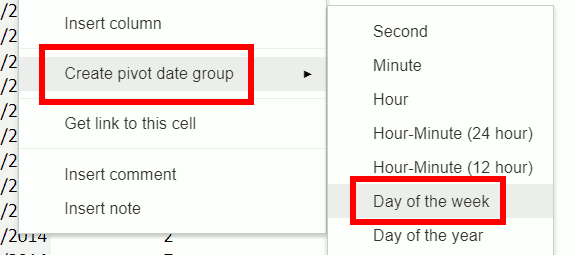
Come over to the column that has the dates in it. Select any one of the days. Right click and do create pivot date group. It doesn’t matter what day you click on in the source table. Google Sheets will give you the option to sort by date or time as long as you left-click on a valid date or time inside the pivot table.

You can do this by week, month, day of the week or even units of time smaller than a day such as hour or minute. Since we are doing Day of the Week, it summarizes all of the data from Sheet1 into Monday, Tuesday, etc. If you have things in this column that aren’t working right, go back to your data and make sure that the dates are valid. There are several different ways to get valid dates and to check and make sure that they’re working. So that’s mostly it. We’ve summarized this data by month with just a few clicks! Now that you have the grouped dates, you create interesting tables like summing by day of the week.


Aditya says:
“Create Pivot Date group” is missing in my google sheet, what to do??
Prolific Oaktree says:
Make sure the dates are valid. You can check by using the ISDATE function.