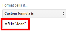
Right now, our custom formula that we built in the previous post is =B1="Joan" and we were applying that formula to column A by using A2:A for the range.
Before formatting the entire row
Custom formula
However, we want to highlight each row, in its entirety instead of just one cell as is shown in this linked Google Sheet.
If you want to learn more about the complex subject of conditional formatting, I have created a course about it over at Datacamp. This is an affiliate link and if you use it to make a purchase I will receive a portion of the proceeds. Thank you for supporting my channel!
Only part of row highlighted
Expanding the Selection
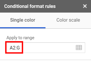
Now, we are going to expand the range used in the “Apply to range” box all the way to column G by entering A2:G into the Apply to range input box. Specifying the range using this syntax will start the range at A2 and expand it down to the end of the spreadsheet and to the right through column G.
Extending the range
Video explanation
Fixing the Formula
If you stop now, it doesn’t change anything. You would think the formatting would extend across the entire row, but it doesn’t. What you need to do is change the formula.
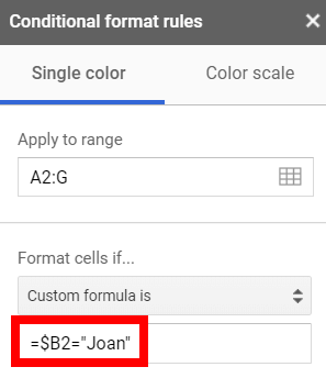
Custom formula with fixed column
Before this change, the formula was incrementing one cell to right each time it calculated, just like any other spreadsheet formula when it is copied to another cell. Now, we have changed the formula from =B1="Joan" to =$B1="Joan". The dollar sign prevents the formula from moving to the right each time it decides if the conditional formatting criteria is being met. You have told your formula to continue looking at the same column for the criteria as it formats each cell. Just like you would if you were inside a spreadsheet cell, you used a dollar sign to indicate that value shouldn’t move when the formula moves.
The Entire Row is Highlighted
It’s working now since we fixed the column reference. Every row that was a sale by Joan has been highlighted.
Custom formula with fixed column
I hope that was helpful. You can take this into your next presentation and wow everyone. You’ll just be amazing;) Have fun with it.
Live examples in Sheets
Go to this spreadsheet for examples of conditional formatting that you can study and use anywhere you would like.
If you’re using Google Sheets and you have two separate columns of data in which you’re looking for matches, there’s a pretty easy way to highlight the matched items. You can also do it the other way around and highlight items that don’t match. You’re typically doing this because your lists are long and you can’t do it visually. However, for this example the lists are purposely small so it’s easy to see.
Matches between two columns are highlighted
Conditional Formatting
We’re going to do it through Conditional Formatting. Go to your menu, then to Format, and select Conditional formatting. The Conditional formatting menu options will pop up on the right-hand side and there’s everything you need right here.
If you want to learn more about the complex subject of conditional formatting, I have created a course about it over at Datacamp. This is an affiliate link and if you use it to make a purchase I will receive a portion of the proceeds. Thank you for supporting my channel!
Menu option for conditional formatting
Rules for conditional formatting
First, apply the conditional formatting to the range which, in this shared spreadsheet (which is also embedded near the end of this page), is C1 to C10. Note that the range is different in the video but the process is the same. You can select the range with your mouse or type it in as C1:C10.
At first, the range should be highlighted because it is set to highlight if it’s not empty. Change this to a custom formula, which is at the bottom. Click on Custom formula is and then it gives you a box that’s waiting for the formula.
Custom formula
You are going to be typing in a formula just like you’re typing into a spreadsheet cell. One of the differences though is now Google Sheets is not going to help you. Once you start typing the function, no helper text will pop up to explain the function. If you want help, type the formula into a cell in the spreadsheet and it’ll help you build it. Then, you can paste it into the custom formula box.
Video explanation
MATCH formula
You want to use a function called MATCH. MATCH is going to look at each cell in the range and check to see if it exists in the other range that you specify. The first parameter that you want, it’s going to do this one cell at a time, is C1. Now type a comma and Sheets will be looking for the range that you want to try to look up C1 in to see if it’s a duplicate. You don’t want this range to shift down every time it evaluates a cell on the right., so use dollar signs before the row numbers to fix the range as such A$1:A$7.
Next, your spreadsheet wants to know if this is going to be an exact match. Enter a 0 (zero) for yes so if it finds exactly Yellow. Now close it off with the parentheses. Your code should look like this:
=MATCH(C1,A$1:A$7,0)
The box that contains this function should have changed from red to blue meaning that the function is now a valid function. It should be working after the box turns blue. You can see it highlighted the color red in green because red is on the list on the left but it didn’t highlight orange because orange isn’t in that list. If you click done, you’ve highlighted everything that exists in the other list.
=ISNA(MATCH(C1,A$1:A$7,0))
If you want to do this the opposite way, and highlight the items in this list that aren’t in the list on the left, wrap your formula in the function called ISNA. The ISNA function is saying – look, if the MATCH function doesn’t work, highlight it. Not if it does work. After the ISNA, put a parenthesis and then go to the very end and close it with the parenthesis.
View of Sheet with ISNA applied
Live examples in Sheets
Go to this spreadsheet for examples of comparing two lists that you can study and use anywhere you would like.
Using a plugin
As an alternative to the options above, you may want a plugin to do the heavy lifting for you. I like to use a plugin called Power Tools. This will give you a menu option with, among other things, several options to deal with duplicates. You can use the plugin to combine or remove duplicated rows.
Dedupe and Compare Menu
Conclusion
After following this tutorial, you should be able to highlight matches or differences between two columns. If you have any questions, feel free to leave a comment below.
Disclosure: This is an independently owned website that sometimes receives compensation from the company's mentioned products. Prolific Oaktree tests each product, and any opinions expressed here are our own.