Leading and trailing white space

Google Sheets – Remove leading and trailing spaces

Leading and trailing white space

If you’re using Google Sheets and you have a column of data like the one in the image with leading and trailing spaces, it can be tricky to clean it up. There may be spaces before some of the letters or spaces after them that you want to get rid of. This tutorial will show you steps to get that done. This process can be just a few steps, but you may have some white space that is more difficult to get rid of and the later examples in this guide will show you how to deal with those.

Regular “space bar” spaces

Trailing white space
Leading white space
Leading white space

If it’s just a matter of getting rid of spaces that are from someone hitting the space bar, then it is pretty easy. If you hit your F2 button or double left-click your mouse in one of the cells, you can see there’s a leading space because the cursor isn’t next to the first character. I you use the left or right arrow key, the cursor will get to the characters, but it starts out to separated by white space. These example images are showing both leading and trailing white space.

Trimmed
White space being trimmed

The four names in the example above all have regular leading and trailing spaces. These can be taken care of with the TRIM formula. That is going to be the quickest option as this is what this function is made for. Copy the TRIM formula down the column and it works…until it doesn’t.

Video explanation

When TRIM doesn’t work

Some white space remaining

The TRIM function worked on the first four examples. If that works on all of your data, great! Leave it there because it’s the easiest to use and maintain. But, once we got to Shannon Rutherford in the example above, it stops working. It’s the same TRIM function, but there’s a leading space that did not go away. What is happening is that there’s a non-breaking space. A non-breaking space is a little bit different from a “regular” space and it’s just not what the TRIM function looks for. The TRIM function is doing its job, but it thinks there is nothing to get rid of. A non-breaking space is special character, number 160 if you are keeping track.

SUBSTITUTE Function
Add the SUBSTITUTE Function

Now we’ve added the SUBSTITUTE function. What the SUBSTITUTE function does is it looks to see if there are any character 160s, which is a non-breaking space, and, if so, changes them into a regular space. Then the TRIM comes along and gets rid of that regular space. So that’s kind of the next level. If you still have leading spaces after using SUBSTITUTE, you might just want to jump to the third level.

CLEAN function
CLEAN function

Add in the CLEAN function and there are three functions wrapped into a formula that should get rid of everything. In this example, it is removing the line break from Jin-Soo Kwon These three functions in combination also trim white space out of the middle so be careful. Make sure that’s what you want.

 Live examples in Sheets

Go to this spreadsheet for and example that you can study and use anywhere you would like.
.5 inch hanging margin

Google Docs | APA or MLA Hanging Indent Works Cited with Template

Objective

If you want to create a works cited page that is APA and MLA compliant in Google Docs, you will need to use hanging indents of 1/2″. Let’s start with a works cited page with no indents as seen below.

No hanging indent
Doc without hanging indents

Steps

First, you need to make sure that you can see your ruler. If you can’t see the ruler, go to View. Show ruler should be checked.

Google Docs ruler
Make sure your ruler is showing

Video explanations

The second thing is, for works cited entries that are more than one line, make sure you have not used the Enter key between the lines. If you have used the Enter key in between lines, Docs is not going to know what lines belong together, so it’s not going to do the indent right.

Next, select all of the text in the area that needs the hanging indents. Then, take your cursor up to the ruler. You’ll see a horizontal line which is the First Line Indent and a triangle which is the Left Indent that are together right now. They act together so just left click on them anywhere and drag them to the right half an inch.
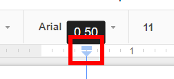
left indent and margin .5
Left indent and margin .5 inch

You’ll know it’s a half inch because that number above the two symbols is going to show you 0.5. This indents everything. We’re halfway there. Now just grab the top part of the two which is called “First line indent”, the little rectangle, and go back to zero. There, you have a hanging indent.
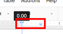
left indent .5 margin 0
Left indent .5 left margin 0

Every entry now is covered by the hanging indents. You will be able to tell because, if there’s a subsequent line like the third entry, it will indent the subsequent line.

.5 inch hanging margin
Doc with hanging indents

Conclusion

So there you go. It’s not too bad once you know how to do it. It’s just learning the trick of how to apply it. I hope that was helpful.

Live Google Doc Template with Hanging Indents

To start with this template, go to File and choose Make a copy.

Data validation menu option

Google Sheets – Create drop downs from a range of data

You may want to create a drop down list in Google Sheets using data that is already in your spreadsheet. This data could change from time to time, and the values in the drop down list will change with it.

Data validation

A drop down with dynamic values can be created in just a few steps. Select the cell(s) that you want the drop down to be in and then go to the Data menu and then Data validation. Keep in mind that some newer spreadsheet programs have a built-in drop-down data type.

Data validation menu option
Menu option for Data validation

Once the Data validation box pops up, choose List from a range. This is where you will select the range that holds the values that you want for the drop down.

List for a range
Chose List from a range

Video explanation

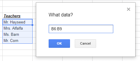
Insert your cursor in the box to the right of List from a range and then highlight the range of cells that contain the values that you need.

To select cells that are not next to each other, just type the cells or cell ranges in separated by commas.

Highlighted range
Highlight the range

When you get back to the Data validation window, the range that you selected will be pre-filled in the Cell range box of the Data validation pop-up window.

Finished drop down
Your drop down list is ready to go!

Click Save and your drop down box with dynamic values is complete.

Follow image below for the live Google Sheet with this data

docs share icon

Data validation menu option

Google Sheets – Create drop downs in less than one minute

You may be looking to give your spreadsheet users a quick drop down from which they select a value. You can create this feature in a few, simple steps. Keep in mind that some newer spreadsheet programs have a built-in drop-down data type.

Data Validation

You start out by going to the Data menu and then selecting Data validation. Note that you have to be on the desktop version of Sheets to create this drop down. There is no Data validation option in mobile Sheets.

Data validation menu option
Menu option for Data validation

Once you have selected Data validation, select the List of items option.

List of items option from drop down box
Choose list of items

Type the different values for your drop down.

Values for drop down

You’re done! This drop down will always be in this cell with exactly the values that you entered. If you want to change the values, you will can go back into the Data validation options and change them from there.

Finished drop down
Finished drop down

Follow image below for the live Google Sheet with this data

docs share icon

Good and bad dates

Google Sheets – How to Sort Dates into Chronological Order

You may already know how to use the SORT function or how to use the menus to sort a list of dates. But, these sorts don’t always work correctly with dates. Dates are notoriously tricky to work within a spreadsheet as can be seen in the linked example file.

Good and bad dates
Good and bad dates

The only hint that Sheets gives you about the validity of your dates is the alignment of the data in the cell. If it recognizes a date, it will be shown as right-aligned. Even the November 6th, 2012 date above is invalid, but it is difficult to tell because the contents fill most of the cell, hiding the fact that it is left-aligned.

In order for a date to work like a number, Google Sheets has to recognize it as valid. If Sheets does not recognize your date, it won’t be able to sort it in relation to any other dates. When Sheets does recognize a value as a date, it converts it to a serial number so that it can use it in formulas.

Check Dates for Validity

So, how do you make sure all of your dates are valid? You can do this using the DATEVALUE function. The DATEVALUE function checks a date to make sure that Sheets thinks it is valid. If the date is valid, it is returned as a serial number representation of that date. If the date is not valid, it returns a #VALUE! error. If you sort the results, all of the #VALUE!s will be together, then you can fix the dates that aren’t valid and try your sort again.

Dates with DATEVALUE being used

Watch the video

Sort Based on Date Values

If you sort your list now, all of the invalid dates are grouped together. Since they have been grouped together, now you can work on fixing each of them until the #VALUE! error goes away. First, highlight the range of data to sort. Be sure to select all of the columns but leave out the header row.

Values to be sorted are highlighted
Highlighted values to sort

After highlighting the range that you want to sort, go to Data validation then Sort range. If you sort without selecting the range, Sheets automatically sorts by column A which is not where your date values are.

Sort range

Sort range

Next, select column B (or whatever columns your dates are in).

Pick the correct column

After sorting, all of your invalid dates are grouped together. As you correct each one, the DATEVALUE formula will change from #VALUE! to the serial number representing that date. After they are all fixed, you’re ready to sort again!

Sorted data
Sorted data before fixing the dates

After fixing
After fixing the dates, before re-sorting

Each date sorts as expected now that every date value has been checked and fixed with the help of the DATEVALUE function.

Sorted data after fixing
Fixed and re-sorted correctly

Keep Your Dates Sorted

If you add new dates to your spreadsheet, there are two methods to keep them sorted. You can either resort them manually as discussed above, or use the StaySorted add-on to automatically sort any new entries.

 Live examples in Sheets

Go to this spreadsheet for examples of sorting dates that you can study and use anywhere you would like.