If you’re using Google Sheets and you are trying to figure out how to put a pop-up calendar date selector inside a cell, it is not very straight forward. We are going to go through a set of steps to show you how.
Purpose
Pop-up calendars can be used to make it easier for a spreadsheet’s users to enter data. Pop-up calendar date selectors can also validate data to give the user a message or reject the cell’s input if it is not a valid date.
Data validation
The pop-up calendar comes as a result of applying data validation to a cell or range. To apply data validation, choose Data -> Data Validation.
Menu option for Data validation
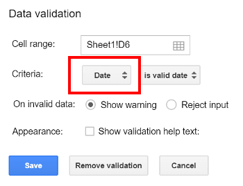
Once you are in the options for data validation, all you have to do is change the criteria to Date. The other options can be left as is for now.
Date criteria selected
Calendar
It may not look like it, but you’re done. You only see the calendar if you double-click in a cell. If other people will be using your spreadsheet, you may want to indicate this so they know that a calendar is there.
If you are using Google Docs to write a document with data from a Google Sheet, you may want to show it as a linked table. If you create the table in Google Docs with no linking, it will not update if the data in the Google Sheet changes. Also, this is double work as the data is already in the Sheet, so re-typing it is a waste of time. Below are instructions on how to embed a live Google Sheet directly into your Google Doc. The table that is created will update with one-click and can be styled however you like.
Create the Sheet
First, you need a spreadsheet created in Google Sheets with the table of data that you want to display in your Google Doc. In your spreadsheet, highlight the range that you want, right-click, and select Copy.
Table to be copied
Paste it into your Doc
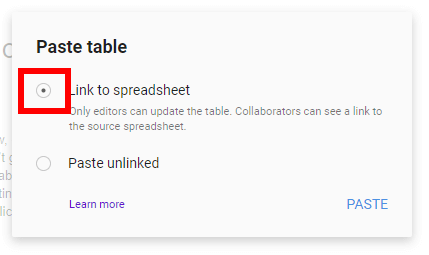
Then, go to the location in your Google Doc where you would like the table to be inserted. Right-click with your mouse and choose Paste. A window will pop-up asking you if you want to Link to spreadsheet or Paste unlinked. Choose Link to spreadsheet and click Paste.
Choose Link to spreadsheet
Oh yes, that’s a live, linked table that you’re seeing.
Google Doc with embedded Sheet
Watch the Video
Working with your embedded table
Updating the embedded table
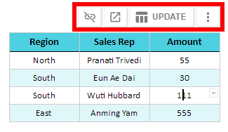
If you want to change the data within the table, you can go back to the Google Sheet to make the changes. When you come back to the Google Doc after making the changes, there will be a new option available to update the table when you right click on the table as shown in the picture below.
Adding rows
If you add rows to your table in Sheets, you may notice that the added rows don’t show up in the linked table in Docs. You will need to go back to the table in Docs after making the change, left click the more button (three vertical dots), and choose Change range.
Option to change the range
Formatting the table
Formatting is probably best done in Sheets, but if you wish to format the table in Docs, you can right click on the linked table in Docs and choose Table Properties. This will bring up several options that will allow you to add bling to your table until you are satisfied.
Table properties
Conclusion
Following the steps above should provide you with an easy way to insert a live, linked spreadsheet into your Google Document. Enjoy!
If you are using Google Slides to create a presentation with data from a Google Sheet, you may want to show that data as a linked table. If you create the table in Google Slides with no linking, it will not update if the data in the Google Sheet changes. Also, this is double work as the data is already in the Sheet, so re-typing it is a waste of time. Below are instructions on how to embed a live Google Sheet directly into your Google Slide. The table that is created will update with one-click and can be styled however you like. Live links to the Slide and Sheet shown in this tutorial are at the end of this article.
Delete the existing text box
Slides wants a blank area for the table. If you have a text box in your slide, delete it to make a nice, big open space.
Text box to be deleted
Watch the video
Create the Sheet
You need a spreadsheet created in Google Sheets with the table of data that you want to display in your Google Slide. In your spreadsheet, highlight the range that you want, right-click, and select Copy.
Table to be copied
Paste it into your Slide
Then, go to the location in your Google Slides where you would like the table to be inserted. Right-click with your mouse and choose Paste. After clikcing, a window will pop-up asking you if you want to Link to spreadsheet or Paste unlinked. Choose Link to spreadsheet and click Paste.
Choose Link to spreadsheet
Oh yes, that’s a live, linked table that you’re seeing.
Google Slide with embedded Sheet
Working with your embedded table
Updating the embedded table
After linking the table, if you want to change the data within the table, you can go back to the Google Sheet to make the changes. When you come back to the Google Slide after making the changes, there will be a new option available to update the table when you right click on the table as shown in the picture below.
Adding rows
If you add rows to your table in Sheets, you may notice that the added rows don’t show up in the linked table in Slides. You will need to go back to the table in Slides after making the change, left click the more button (three vertical dots), and choose Change range.
Option to change the range
Conclusion
Following the steps above should provide you with an easy way to insert a live, linked spreadsheet into your Google Slides. Enjoy!
As of April 2018, checkboxes can be inserted using Insert, Checkbox from the menus. This tutorial is still relevant however, if you would like to use drop-downs with other types of characters.
If you want a way to choose yes/no in Google Sheets, using a checkmark can be a good way to do it. While it is not a built-in function, there is a way to create a checkbox drop-down in Google Sheets as shown in this linked Google Sheet. The method is a bit of a workaround, but it does end up giving you a drop-down with the option of a box with a checkmark in it or a blank box. Keep in mind that some newer spreadsheet programs have a built-in drop-down data type. The steps below will get you there quickly.
Note that this video discusses both dropdowns and checkboxes.
First Step – Data Validation
Click on the Data menu option and then Data Validation.
Menu option for Data validation
Once the Data validation window pops up, choose List of items from the criteria drop-down box.
Choose list of items
Pick from a few different symbols
Copy and paste the two checkmark symbols below. These will be the two options that show in the drop-down list. If you would like other symbols, consider using the Insert Special Characters add-on for Google Sheets. Below are two easy, intuitive symbols.
✓,𝤿
Following are more options you can use. Note that you can have the user click a checkmark for yes, and leave the drop-down empty for no if you want to just use a checkmark not the empty box.
⌧☑✅✓✔???
End result
Keep the rest of the options at their defaults and choose save. You now have a check box!
Check box drop down
Live examples in Sheets
Go to this spreadsheet for examples of checkboxes that you can study and use anywhere you would like.
When you’re working with data in a spreadsheet, there are often duplicate values that need to be considered. This tutorial will show you how to highlight the repeated items in a few easy steps.
First, highlight the column or row that you want to evaluate.
Click Format in the top menu then Conditional formatting…
Menu option for conditional formatting
The Conditional Formatting menu option will pop up a Conditional format rules menu on the right side of the screen (on the desktop version of Sheets).
If you want to learn more about the complex subject of conditional formatting, I have created a course about it over at Datacamp. This is an affiliate link and if you use it to make a purchase I will receive a portion of the proceeds. Thank you for supporting my channel!
Rules for conditional formatting
Click the plus sign to begin adding the rule. In the drop-down menu for Format cells if choose the last option which is Custom formula is.
Last menu option is custom formula
In the box that appears below Custom formula is enter =COUNTIF(A:A,A1)>1. Note that you have to start the formula with a = sign just like any other spreadsheet formula. If you were highlighting a row instead of a column, specify the row as 1:1 if the row were the 1st row. If you are not familiar with COUNTIF, learn how to use it here.
This will start at A1 and check to see if the value in A1 occurs more than once in the selected range. Then, the conditional formatting goes to the next cell, A2, and so on, until it gets to the end of your specified range. Now, all of the duplicates in your list are highlighted.
The A:A may seem a little strange but this is a method of specifying an entire column no matter how many rows are used.
Result with highlights duplicated
Video explanation
Live examples in Sheets
Go to this spreadsheet for examples
of highlighting duplicates that you can study and use anywhere you would like.