Google Sheets – Count cells containing specific text

If you’re using Google Sheets and you want to count the occurrences of a certain letter or word, there’s a pretty easy function that you can use.

Looking for a word and only that word

In this first set of data in the image above and also in this linked spreadsheet, we will be counting any cells that contain the word “Yellow” and only that word. To count the occurrences of the word yellow in the range B2 to B9 you can use the count COUNTIF function as such: =COUNTIF(B2:B9,"yellow"). It performs a conditional count. In this case, only if the cell or ranges of cells is equal to Yellow. Yellow is not case-sensitive so this is going to pick up three instances even though B7 is not capitalized. If the COUNTIF technique is doing everything you need, then you’re done and there is no need to try anything more involved.

Looking for a word occurring anywhere a cell

COUNTIF with wildcard

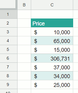
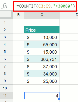
Looking at this second set of data, things will get a little bit more complicated. We are looking for a certain word that occurs anywhere in any of these cells. First, you want to use COUNTIF again and give it a range =COUNTIF(C2:C9, "*Yellow*"). For this example, the range will be C2 to C9. If it has the word yellow and anything before which is what the asterisk means, and anything after it which is the second asterisk, then it should be counted. It just has to have yellow in some part of it. Anything can be nothing so it can start or end with yellow too. This function is also counting 3 because of the yellow plane, the yellow car, and the little yellow boat.

Case-Sensitivity

The COUNTIF function is not case-sensitive. To count cells with specific capitalization, follow the second example in this tutorial.

Using a plugin

As an alternative to the options above, you may want a plugin to do the heavy lifting for you. I like to use a plugin called Power Tools. This will give you a menu option with, among other things, advanced Find and Replace features. This will give you a list of all the occurrences of a word in your spreadsheet, but it won’t give you a count of them. Depending on the size of the spreadsheet, this may be the preferable option.

The Find and Replace Menu
Find and Replace Menu

I hope that was helpful and now you know the formula for counting any occurrences of any word that you’re looking for.

Β Live examples in Sheets

Go to this spreadsheet for examples counting specific text that you can study and use anywhere you would like.

Disclosure: This is an independently owned website that sometimes receives compensation from the company's mentioned products. Prolific Oaktree tests each product, and any opinions expressed here are our own.

COUNTA

Google Sheets – Count cells that are not blank

If you’re using Google sheets and you want to count the number of cells if they’re not blank, there are a couple different ways to do it and some complications that you might run into.

COUNTA usually works

I’m going to show you the easy way and a little bit harder way if you run into trouble. Let’s use COUNTA with the range from B3 to B9. The syntax, as also shown in the image above and the linked Google Sheet, is =COUNTA(B3:B9). This is the easy, straightforward way that’ll probably work most of the time. COUNTA is a built-in function. It will count any cell with a value and within the specified range. If that works for you, then you’re done. Don’t worry about it.

Video explanation

Longer formula
Longer formula

But, if we go to column C, things can get a little bit more complicated. This column looks like it has the same number of values, right? However, the COUNTA has the same range but is picking up seven instead of six. That’s happening because I snuck a blank space in C5. You may want to count this blank space since it is technically a value even though you cannot see it. If that’s the case, then then you’re done. COUNTA will work and the result is seven.

Longer function to not count white space

But, you may not want to count this blank cell. Accordingly, you may want to count what appears to have data in it, and you don’t really consider an empty space to be data. If this is the case, you have to use a more complicated formula. The function in cell C12, =SUMPRODUCT(--(LEN(C3:C9)>0)) is adding everything when the LEN function returns something greater than zero. LEN is counting the number of characters. The LEN function will not count the spaces that don’t really have any characters and, if that’s what you want, then that’s the way to get it done.

Now you have two different choices to count the number of cells that are not blank. A simple COUNTA for cells with no values at all, and the longer alternative, LEN, to exclude the empty spaces from the count.

 Live examples in Sheets

Go to this spreadsheet for examples of adding and subtracing days, months, or years that you can study and use anywhere you would like.
Column of numbers

Google Sheets – Count cells greater or less than an amount

If you’re using Google Sheets and you have a column of data in which you want to count the number of items that are greater or less than a certain amount, there are a couple of small nuances to it, but generally, it’s pretty easy.

Column of numbers
Column of numbers

Column of numbers with COUNT function
Numbers with a count

To perform this count using the data in the images above, we’ll be using the COUNTIF function in cell C11. This is a function that’s going to count a range if a certain criteria is met.

  • Place your cursor in cell C11 and type =COUNTIF(C3:C9,">30000"). The C3 is the start of the range and C9 is the end.
  • After you type the range into the function, enter a comma. That lets Google Sheets know that you are done with the range.
  • Then, enter the criteria surround by quotes. We’re going to do anything greater than 30,000. Don’t put a comma in your 30000 or it’s going to think it’s text instead of number.

After you entered the formula, you can see there are four items over 30,000 and this counted them. Easy as pie.

Video explanation


 Live examples in Sheets

Go tothis spreadsheet for examples of that you can study and use anywhere you would like.

adding only days

Google Sheets – Add or subtract days months or years to a date

If you’re using Google Sheets and you want to add or subtract days, months, or years to a date, we’ll step through how to do that.

Add or Subtract Just Days

Working with just days is simple because of the way dates are stored in Google Sheets. All you do is take the starting day and then you add the value to it. We’re going to add the value that’s in E5 to B5 and it steps that value forward by nine days.

adding only days
Adding only days

Video explanation

Add or Subtract Days, Months, or Years

Things get a bit trickier if you want to add years, months, or days because dates are stored just as serial numbers. They are incremented only by days and then Google Sheets figures out what that total is in days, months, and years. In order to add months or years instead of days, you have to wrap this in the DATE function as shown in this linked file used to create this post. The DATE function tells Google Sheets that we are looking at a date and that date has three values. Start your formula with an = sign like you always do. Your inputs are the month, and day, and year that we’re starting with. The formula to add the amounts in row 6 of the image is

=DATE(YEAR(B6)+C6,MONTH(B6)+D6,DAY(B6)+E6)

This is going to take B6 and add the number of years, months, and days to it that are in this table. This adds a year but it also added 11 months and 27 days so it almost added two entire years. That’s why it’s 2018. The function is smart enough to know the different numbers of days in each month and if you go over 12 months, it increments the year by one. If copy and paste the formula down the column, you see that it’s working in all these situations. Just for fun, we’re gonna take a negative 46 in the last example to perform subtraction. That works as well. It took you back in time to 1932.

adding days months years
Days, months, and years

I hope that helps if you’re using a spreadsheet to add or subtract days, months, or years. For another post about working with dates, learn how to sort them as they can be quite picky.

 Live examples in Sheets

Go to this spreadsheet for examples of adding and subtracing days, months, or years that you can study and use anywhere you would like.

Using a Plugin to Work with Dates

If you are doing a lot of work with dates, you can a plugin called Power Tools to, among other things, split dates and times into separate cells.

The Split Date and Time Menu
Split Date and Time Menu

Disclosure: This is an independently owned website that sometimes receives compensation from the company's mentioned products. Prolific Oaktree tests each product, and any opinions expressed here are our own.

Leading and trailing white space

Google Sheets – Remove leading and trailing spaces

Leading and trailing white space

If you’re using Google Sheets and you have a column of data like the one in the image with leading and trailing spaces, it can be tricky to clean it up. There may be spaces before some of the letters or spaces after them that you want to get rid of. This tutorial will show you steps to get that done. This process can be just a few steps, but you may have some white space that is more difficult to get rid of and the later examples in this guide will show you how to deal with those.

Regular “space bar” spaces

Trailing white space
Leading white space
Leading white space

If it’s just a matter of getting rid of spaces that are from someone hitting the space bar, then it is pretty easy. If you hit your F2 button or double left-click your mouse in one of the cells, you can see there’s a leading space because the cursor isn’t next to the first character. I you use the left or right arrow key, the cursor will get to the characters, but it starts out to separated by white space. These example images are showing both leading and trailing white space.

Trimmed
White space being trimmed

The four names in the example above all have regular leading and trailing spaces. These can be taken care of with the TRIM formula. That is going to be the quickest option as this is what this function is made for. Copy the TRIM formula down the column and it works…until it doesn’t.

Video explanation

When TRIM doesn’t work

Some white space remaining

The TRIM function worked on the first four examples. If that works on all of your data, great! Leave it there because it’s the easiest to use and maintain. But, once we got to Shannon Rutherford in the example above, it stops working. It’s the same TRIM function, but there’s a leading space that did not go away. What is happening is that there’s a non-breaking space. A non-breaking space is a little bit different from a “regular” space and it’s just not what the TRIM function looks for. The TRIM function is doing its job, but it thinks there is nothing to get rid of. A non-breaking space is special character, number 160 if you are keeping track.

SUBSTITUTE Function
Add the SUBSTITUTE Function

Now we’ve added the SUBSTITUTE function. What the SUBSTITUTE function does is it looks to see if there are any character 160s, which is a non-breaking space, and, if so, changes them into a regular space. Then the TRIM comes along and gets rid of that regular space. So that’s kind of the next level. If you still have leading spaces after using SUBSTITUTE, you might just want to jump to the third level.

CLEAN function
CLEAN function

Add in the CLEAN function and there are three functions wrapped into a formula that should get rid of everything. In this example, it is removing the line break from Jin-Soo Kwon These three functions in combination also trim white space out of the middle so be careful. Make sure that’s what you want.

 Live examples in Sheets

Go to this spreadsheet for and example that you can study and use anywhere you would like.