Using Google Sheets for conditional formatting based on a range’s own values is simple. Formatting based on another range of cells’ values is a bit more involved. Following are step-by-step instructions to format a range of cells using values in another range of cells.
What is conditional formatting
Conditional formatting is used to highlight to the reader of the spreadsheet certain values that meet certain criteria. It can be used to show items over/under a certain amount, later/earlier than a certain date, or only the widgets sold by Joan.
Video explanation
If you want to learn more about the complex subject of conditional formatting, I have created a course about it over at Datacamp. This is an affiliate link and if you use it to make a purchase I will receive a portion of the proceeds. Thank you for supporting my channel!
Conditional formatting based on another cell
Our objective in this example is to highlight all of the dates on which Joan had a sale.
Select the range that you want to have highlighted. Even though you are going to be referencing another range of cells, you still only need to select the range that you are going to be formatting. In this example, we’ll be highlighting the date column.
Two columns, one highlighted
Click Format in the top menu then Conditional formatting…
Menu option for conditional formatting
The Conditional Formatting menu option will pop up a Conditional format rules menu on the right side of the screen (on the desktop version of Sheets).
Rules for conditional formatting
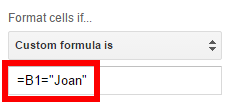
Click the plus sign to begin adding the rule. In the drop-down menu for Format cells if choose the last option which is Custom formula is.
Last menu option is custom formula
In the box that appears below Custom formula is enter =B1="Joan". Note that you have to start the formula with a = sign just like any other spreadsheet formula. Also, note that you need to surround the word Joan with “s since it is a word instead of a number.
Custom formula
Now you have the sales data with dates highlighted on which Joan made sales.
After conditional formatting
Extending to the entire row
If you want to highlight the entire row based on the value of one cell, continue reading here.
Live examples in Sheets
Go to this spreadsheet for examples of conditional formatting that you can study and use anywhere you would like.
Yahoo Mail does not let you view attachments and print them like other email programs without saving them first. In order to view attachments full screen and print them, you are forced to save them onto your computer and then open them. This creates extra steps and leaves the clutter of all of your past attachments in your computer’s file system
Typical email preview with the paperclip icon indicating an attachment
Description
The files are shown as colored square icons at the bottom of your email message. If you hover your mouse over the icon, you get the option to download the file. Click on the white letters that say download at the bottom of the icon.
Icon showing attachment
Video explanation
The next step is where the trouble starts. Instead of the document showing when you click on it or giving you the option to open it, you only have the option to save or cancel. This is assuming that you are using Google Chrome. The Edge browser may show slight variances in these two options but it still won’t let you open the file.
Save or cancel, no open!
Why it happens
The reason this is happening is because of the browser that you are using. Google’s Chrome and Microsoft’s Edge browser do not have the option to open files without saving them first. However, both Firefox and Internet Explorer browsers do let you open files. First, we will look at Internet Explorer.
Solution 1
The easiest solution is to use Internet Explorer. This program should already be installed on almost any Windows computer. You can find it on Windows 10 by going to all programs, Windows Accessories, Internet Explorer.
Internet Explorer in the Start Menu
Next, open up Internet Explorer and click on the colored rectangle icon to view your attachment. Now you get the option to OPEN it. Viola! If you open it, you can view and print it without saving.
Internet Explorer gives you the option to open the file
Solution 2
For a more secure solution, you can download the Firefox browser which will give you an up-to-date browser that has constant security and feature updates. Firefox is developed and maintained by the non-profit Mozilla Foundation.
Calculating age in a spreadsheet can be a painful process using many of the formulas floating around the web today. Dates act strangely in spreadsheets so care must be taken when working with them. Fortunately, calculating age can be done much easier using a single function in Google Sheets called DATEDIF. The DATEDIF function will return the difference between two dates in days, months, or years. Using these units in combination can get you a variety of output options.
Use the TIMEDIF add-on if you are working with dates and times.
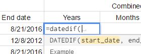
Syntax
=DATEDIF(start_date,end_date,unit)
start_date Date at which to start the calculation
end_date Date at which to end the calculation
unit Type of output. Choices are “Y”,”M”,”D”,”YM”,”YD”, or “MD”.
Y – Number of whole years elapsed between start and end dates
YM – Number of months elapsed after the number of years shown with the “Y” unit. Will not exceed 11.
YD – Number of days elapsed after the number of years shown with the “Y” unit. No matter how many days after the last year, starts counting after end of last full year and is never over 364.
M – Number of whole months elapsed between start and end dates
MD – Number of days elapsed after the number of months shown with the “M” or “YM” unit. Can’t go higher than 30.
D – Number of whole days elapsed between start and end dates
Watch the video
Examples
Follow image below for the live Google Sheet with this data
Live examples in Sheets
Go to this spreadsheet for examples of calculating age that you can study and use anywhere you would like.
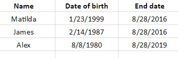
Let’s say that you have three columns of data. As long as you have start and end dates, you are ready to go.
Columns for name, start date, and end date
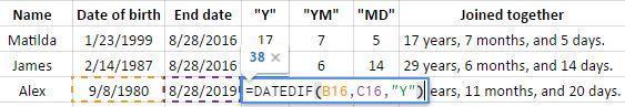
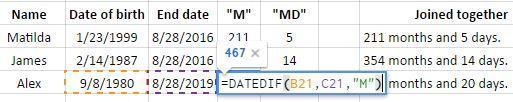
Now add 4 columns to the right for the DATEDIF formula with “Y”, “YM”, “YD”, and a column with them joined together. Remember that all of these are in the live Google Sheet shared above. The Y, YM and MD are used as the “unit” in each respective column. The “Y” column is showing the person’s age in years. The “YM” is showing the number of months that have elapsed since the last year shown. The “MD” column is showing the number of days that have elapsed since the last whole month.
Y, YM, and MD units added
There are other types of units as well. This next example uses M and MD. Note that the number of months goes over twelve since the years are not in the formula’s output. The column using MD as the unit is the same calculation as above.
M and MD units
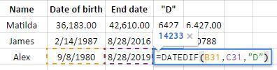
This last example uses just the D unit. If you are just using this function to calculate days, it would be easier to use a subtraction formula for the number of days or the DAYS function. Dates in spreadsheets are actually stored as integers so they can easily be added and subtracted. The last column, which is unlabeled, contains a subtraction formula.
Just days
If you want to calculate and age and have it always be current when you open the spreadsheet, consider using the function called TODAY as your end date. TODAY returns the current day.
To just calculate the number of fractional years between two dates, consider using the YEARFRAC function.
Google Sheets allows you to build pivot tables to summarize large data sets. When building the pivot tables, you can also add fields that perform calculations on the data once it is in the pivot tables as shown in this live Google Sheet. These calculated fields are a must-have in certain situations as you may want to add/subtract/multiply/etc summarized data from the pivot table that doesn’t exist in the original data being pivoted. For example, if you have a table of salaries and years of college each employee attended, you may want to calculate the return for each year of college. To do this, you would first summarize the data by average salary for each group, then perform the division to arrive at the average after the data is summarized.
This tutorial assumes that you have completed your Pivot Table and know how to use it. See this video if you need some basic help on Pivot Tables.
If you need a primer on Pivot Tables, this video will walk you through them.
The “Salary per year of college” column above is a Calculated Field that is the quotient of the first and second column as seen in the Pivot Table parameters below which can be seen on the right-hand side of your browser screen when you select a field inside the Pivot Table.
Pivot table parameters used to create this Pivot Table
Pivot table calculated fields can allow you to leave the original data in its raw, untouched form. Then, you can use the pivot table to present the data however you would like without changing the original data given to you. Further, it is easier to calculate the average after summarizing the data. It is the average of the summarized data that you are after.
To insert a calculated field, you should first build your pivot table. Then, once you have the data pivoted, you can insert the calculated field using the options on the right side of the screen. As of the date of this writing, this can only be done on the desktop browser version of Sheets.
Live examples in Sheets
Go to this spreadsheet for an example of a pivot table with a calculated field that you can study and use anywhere you would like.
If you’re using Google sheets and you have a list of amounts that you want to sum or count based on the background color of the cells, there’s no built-in function to do it. However, there are a relatively easy set of steps to make your own functions to get it done. You’ll be able to count based on cell color and you’ll be able to sum as well.
**This technique has been updated. There is a new YouTube video showing an easier way with this Sheet**.
Custom formulas in action
Light blue cells being summed and counted by color
Count by cell color
If you look in the live spreadsheet, you will see the custom formulas being used for summing and counting by cell color. The counting is done by a formula with the nice little name of countColoredCells which takes the range and cell with the background color that you want as its two inputs. You want to count B4 through B9 and you want to count the number of cells that have the background color used in cell B8, which is the light blue cell with the dotted line around it.
Formula for count by cell color
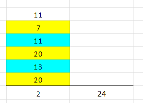
If you change the second parameter above from B8, a light blue cell, to B5, a yellow cell, the result would be 3 because there’s three yellow cells.
Sum by cell color
sumColoredCells is returning a 24 which is the sum of all the light blue cells. It is similar to the count function – it is summing the colored cells in B4 through B9 that are formatted like B8.
Formula for sum by cell color
Creating custom formulas
How do we make these functions and any other custom function that you’re so inclined to write? First, go to Tools and you go to Script editor... Don’t worry, we’re just going to copy and paste code below. The code for countColoredCells was obtained from this page at iGoogleDrive.
 /**
* @param {range} countRange Range to be evaluated
* @param {range} colorRef Cell with background color to be searched for in countRange
* @return {number}
* @customfunction
*/

function countColoredCells(countRange,colorRef) {
  var activeRange = SpreadsheetApp.getActiveRange();
  var activeSheet = activeRange.getSheet();
  var formula = activeRange.getFormula();

  var rangeA1Notation = formula.match(/\((.*)\,/).pop();
  var range = activeSheet.getRange(rangeA1Notation);
  var bg = range.getBackgrounds();
  var values = range.getValues();

  var colorCellA1Notation = formula.match(/\,(.*)\)/).pop();
  var colorCell = activeSheet.getRange(colorCellA1Notation);
  var color = colorCell.getBackground();

  var count = 0;

  for(var i=0;i<bg.length;i++)
    for(var j=0;j<bg[0].length;j++)
      if( bg[i][j] == color )
        count=count+1;
  return count;
};
And this code for sumColoredCells was obtained from the same blog, but a different page.
 /**
* @param {range} sumRange Range to be evaluated
* @param {range} colorRef Cell with background color to be searched for in sumRange
* @return {number}
* @customfunction
*/

function sumColoredCells(sumRange,colorRef) {
  var activeRange = SpreadsheetApp.getActiveRange();
  var activeSheet = activeRange.getSheet();
  var formula = activeRange.getFormula().toString();
  formula = formula.replace(new RegExp(';','g'),',');


  var rangeA1Notation = formula.match(/\((.*)\,/).pop();
  var range = activeSheet.getRange(rangeA1Notation);
  var bg = range.getBackgrounds();
  var values = range.getValues();

  var colorCellA1Notation = formula.match(/\,(.*)\)/).pop();
  var colorCell = activeSheet.getRange(colorCellA1Notation);
  var color = colorCell.getBackground();

  var total = 0;

  for(var i=0;i<bg.length;i++)
    for(var j=0;j<bg[0].length;j++)
      if( bg[i][j] == color )
        total=total+(values[i][j]*1);
  return total;
};
Script editor
After you go to Tools then Script editor, you come up with a blank screen. But if you don’t, just do a new script file. Paste the code into the blank window. Repeat for each code section above and name them countColoredCells and sumColoredCells. For each file, the script editor puts the “.gs” at the end of the file name which indicates that it is a Google Script. After you make these two, save them, come back to your spreadsheet, type in the formulas, and it should work for you. See the video and live spreadsheet for further clarification.
Watch the video
Live examples in Sheets
Go to this spreadsheet for examples of counting cells by cell color that you can study and use anywhere you would like.
Using a plugin
As an alternative to the technique above, you may want a plugin to do the heavy lifting for you. I like to use a plugin called Power Tools. This will give you a menu option with, among other things, the ability to run functions by color.
Functions by Color Menu
Disclosure: This is an independently owned website that sometimes receives compensation from the company's mentioned products. Prolific Oaktree tests each product, and any opinions expressed here are our own.