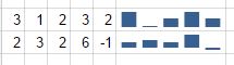
sparklines ymin ymax

Line graph options for Sparklines in Google Sheets with Examples

Sparklines, as seen in the overview post on sparklines, are quick, simple charts that can be inserted into the cell of a spreadsheet created with Google Sheets.  One of their strengths is their simplicity.  However, there are several options that can be used to expand their functionality.  Below, we focus on the options available for use with the line graph type of sparkline.

Line graph options

xmin sets the minimum value along the horizontal axis (not shown)

xmax sets the maximum value along the horizontal axis (not shown)


ymin sets the minimum value along the vertical axis.

ymax sets the maximum value along the vertical axis.

sparklines ymin ymax

color sets the color of the line

empty how to treat empty cells

  • zero give the cell a value of zero for the sparkline
  • ignore ignore the cell, rendering the chart as if it does not exist
  • Note in the image that the “ignore” option behaves the same as not designating this option at all.

Video explanation

sparklines empty options shown with different choices

nan how to treat cells with non-numeric data

  • convert let Sheets try to convert the character(s) in the cell to a number. Good luck on this one.
  • ignore ignore the cell, rendering the chart as if that value does not exist
  • Note in the image that the “ignore” option behaves the same as not designating this option at all.

sparklines nan graphs with different options shown

rtl changes the direction of the chart from left-to-right to right-to-left

  • true The direction of the chart is flipped
  • false The direction of the chart stays the same
  • Note in the image that the “false” option behaves the same as not designating this option at all.

sparklines linegraph with different rtl options specified

linewidth specifies the thickness of the line in the chart

sparklines linechart with different linde widths specified

Follow image below for the live Google doc with sparklines

docs share icon

sparklines no options

Sparklines in Google Sheets – How and when to use them


Sparklines can be added to Google Sheets to act as miniature charts to show trends in data.  They are simpler than Charts but not as versatile.  If you have ever tried to insert a decent chart into a spreadsheet, you can appreciate the simplicity of using Sparklines.

More specific sparkline articles…

Video explanation


To insert a Sparkline, you must use a formula as there is no Sparkline function in the menus.  The syntax is

=SPARKLINE(data,[options])

Using the formula above on a simple data set with no options specified would result in simple Sparklines charts as shown below.

sparklines no options

If you wish to make Sparklines charts that look different than the simple line chart, there are many options available.  Be careful when designating the type of chart as the syntax deviates from typical syntax used when creating spreadsheet formulas, or at least it is different from typical Excel syntax.  Prepare for curly braces and lots of commas and quotes…


Chart types

Line

The default option for Sparklines, the same as shown above.  There is no need to specify this as it would be redundant.  See more information on line chart options in this post.

=SPARKLINE(A1:E1,{"charttype","line"})

Bar

This options makes a “stacked bar chart”.

=SPARKLINE(A5:E5,{"charttype","bar"})

sparklines charttype bar2Column

Make a chart with columns representing the values.  See more information on line chart options in this post.

=SPARKLINE(A5:E5,{"charttype","column"})

sparklines chartype column

WinLoss

Shows only two different outcomes i.e, true/false, thunder/lightning, peanut butter/jelly.  OK, maybe only one of those was a good example.  See more information on line chart options in this post.sparklines chartype winloss 

=SPARKLINE(A13:E13,{"charttype","winloss"})


Follow image below for the live Google Sheet with sparklines

docs share icon

sheets insert drawing menu

Text boxes in Google Sheets – How and when to use them

Inserting a text box into Google Sheets

As discussed in this post, there are many times when a text box is a great solution for displaying large pieces of text in a spreadsheet. Inserting a text box into Google Sheets is possible, but finding out how is not readily apparent. If you have a need for a text box in your data, go to Insert -> Drawing.

sheets insert drawing menu

After selecting Drawing, the Insert Drawing options appear below. Select Text box, which is the second from the right.

sheets insert text box

Once you select insert text box, you will be able to type inside a rectange as shown below. You can also change the border, background color, and text styles. 

insert drawing text box

This is all well and good. If you knew exactly what text you wanted to type and insert and you knew you were never going to change it, then you are done and it was easy. However, in the real world, you never know exactly what you are going to type and you often need to add and delete text. Modifying text, while not terribly hard, is not as easy as it should be. You have to double click on the box, wait for another window to pop-up, and then start typing. Having said that, it’s still easier than typing the content into cells, merging and applying text wrap. It’s just not quite as easy as using a text box in Excel.

Watch the video

comment note menu

Google Sheets – Comment vs Note and how to use them

Google Sheets has recently enhanced its cell commenting ability to include the option of inserting a “Note” or a “Comment.” The differences between the two are not obvious. Following is an overview of what they do and how to choose which one you should use. Follow along with the linked Google Sheet used to create this article.

Both comment and note can be selected by right-clicking on the cell (if you’re using a mouse on a Windows PC).

comment note menu

Use the Note function to leave a simple note in the cell just like you would with Excel’s comment function. With Note, you can simply add information about the cell. Only use this if it doesn’t make sense to add the note directly into the cell. Notes can be helpful, but if they are not needed, they add unneeded complexity. Often, users will overlook notes and only notice information that is typed into cells, so use them only when called for.

google sheets note

Video explanation

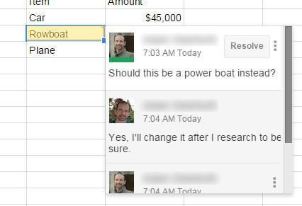
The Comment functionality is Note on steroids. Notes are usually sufficient if one user is creating and viewing a spreadsheet. However, if you have multiple users, especially in different physical locations, the Comment functionality can be very helpful. It enables users to have a back and forth conversation about a cell without altering its contents. The Comment functionality can be especially useful in a supervisor/staff relationship where one person is reviewing another’s work.

Google Sheet Comment

In summary, use the note function when you want to leave a quick note and nothing else. Use comment if you want to start a conversation with someone else about a cell.

 Live examples in Sheets

Go to this spreadsheet for examples of comments and notes that you can study and use anywhere you would like.

protect cells right click

Google Spreadsheets – How to protect cells and ranges of cells

Google has a feature for their spreadsheets that allows you to protect a cell or range of cells from being edited.  The protection is granular and can be customized to the point where you can choose exactly who can and cannot access cells.  The embedded video at the end of this post shows how to do this.  Here are the steps.

  • Highlight the cells or range of cells that you want to protect
  • Right-click and choose “Protect range…”

protect cells right click

Video explanation

  • After choosing Protect range, you have the option of naming the range or you can leave it as is.  Note that you can also protect an entire Sheet (or Tab) from this dialog box as well.  In the screen shot below, I will name the range Management Only to denote that only the people that boss you around are allowed to modify these cells.
  • Use the dialog on the right hand side of your screen to adjust the specifics.
  • Specify a cell or range of cells here, give it a name, and decide who can and who cannot have access.

protect cells and ranges options

  • Note that you can only set permissions for specific users if they have already been invited to view the spreadsheet before you perform this function.
  • You’re done!