If you’re using Microsoft’s Sway and you want to insert an Excel spreadsheet, there’s just a couple easy steps to do it.
The title of your Sway
Create a new Sway and give it a title. I’ve called this one Embedding an Excel Spreadsheet.
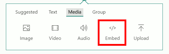
Choose the media group
Next, click the plus sign to add more content. Choose the Media group then click the Embed option.
Choose the embed option
Video explanation
Create a new Excel workbook
Upload an existing Excel workbook
Sway is now waiting for the embed code. You need to get the code from Excel after you’ve uploaded it to OneDrive (or created it online to begin with). So, assuming you’ve uploaded your Excel flle, we’re going to step forward from that point. If you haven’t done that, you need to open up OneDrive and upload it.
Embed option in Excel online
In the online Excel workbook, go to Share and embed and the code is ready at the bottom of the next window. You will be presented with a screen to select different parts of your spreadsheet, leave it at the default for now. Copy the embed code from your clipboard and go back to your Microsoft Sway. Go to the box waiting for your input, and paste the code.
Sway card with embed code
You’ve embedded that Microsoft document. This is live. If you were to update this in Excel, this document that’s showing here would be updated. You can also interact with this document to a certain extent with the icon lower right hand corner. You can download it or print it.
If you’re using Microsoft’s Sway and you want to embed a Google Doc, there’s just a couple easy steps to do it.
The title of your Sway
Create a new Sway and give it a title. I’ve called this one Embedding a Google Doc.
Choose the media group
Next, click the plus sign to add more content. Choose the Media group then click the Embed option.
Choose the embed option
Video explanation
https://www.youtube.com/watch?v=dQT1h2Ph0CY”
Publish your Doc to the web
Click the publish button
Sway is now waiting for the embed code. You need to get the code from your Google Doc by going to the document’s File menu and choosing Publish to the web. Once in the Publish to the web page, you need to click the blue Publish button one time to open up the Doc. After you have clicked Publish, you can highlight the embed code and copy it to your clipboard.
Embed option in Google Docs
Go back to your Microsoft Sway. Go to the box waiting for your input, and paste the code.
Sway card with embed code
You’ve embedded that Google Doc. This is live. If you were to update this in Docs, this document that’s showing here would be updated. You can also interact with this document to a certain extent with the icon lower right hand corner. You can download it or print it.
If you want to track your employees’ time, there is an easy way to do it using Google Sheets that does not involve complicated formulas or macros. This technique will also have the ability to calculate an overnight shift. The linked file that can be copied into your own Drive and used as a template.
Data validation
One of the most difficult things when working with dates and time in Sheets is getting them in the cells correctly. A protection against that, data validation, can be used to reject invalid inputs.
Click on the Data menu option and then Data Validation.
Menu option for Data validation
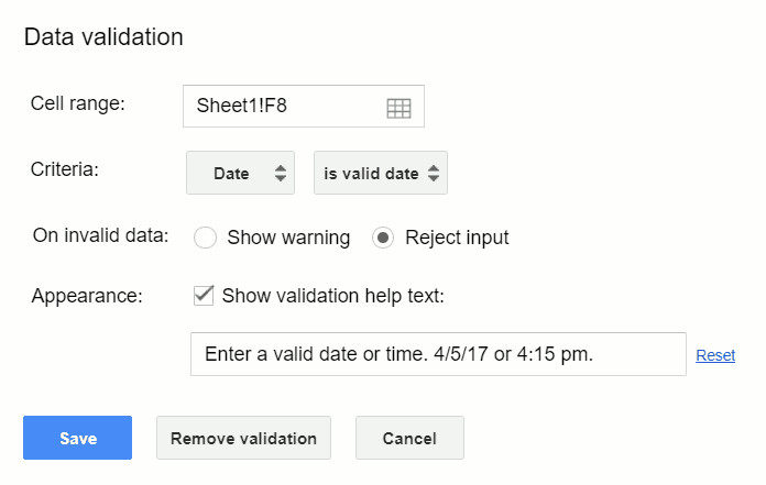
Once the Data validation window pops up, complete it with the parameters in the following pictures including choosing Date from the criteria drop-down box and rejecting invalid input with a message.
Choose date and is valid date
This will set data validation to show the message “Enter a valid date or time” if an invalid date is entered. Times are covered under the date formatting as card card-body bg-light so this data validation is also going to work if it’s a time. Now, if a user enters a date or time that Sheets doesn’t recognize as such, they will get an error message letting them know. There are several different ways to enter a date using a valid format, but there’s infinitely more ways to screw it up. You could do 2-20-18. You could type out February. But, as long as it’s valid, this timesheet will accept it.
The same thing is going to happen with time. If it’s 5:43 and the person types 5 43 in hits enter, it’s not going to work. You have to have a number, a colon, and a number. If you want seconds, do another colon and two digits after that such as 5:43:22.
The formula
Once the validation of the dates and times is set up correctly, the spreadsheet is ready for a start day and time and an end day and time. This formula is going to calculate the hours. So this formula is going to look a little complicated at first, but it’s really not too bad.
As seen in the shared sheet, this formula takes the row it is on and subtracts it from the row above it. To do arithmetic with these dates and times, Sheets has to convert them into a value first. That is what the DATEVALUE and TIMEVALUE functions are doing. The result will be a fraction of a day so multiply that by 24 and that gives you the number of hours worked. Every other row, you want to put in this formula.
If this person takes breaks, just repeat the same formula. If you want to make this longer, just copy and paste it down as many times as you want.
After following this tutorial, you should be able to create a time sheet to track the hours of your empoyees. If you have any questions, feel free to leave a comment below.
Live examples in Sheets
Go to this spreadsheet for examples of the time sheet that you can study and use anywhere you would like.
If you’re using Google sheets and you have a lot of cells that have data in them, you may be trying to figure out which ones have formulas and which ones don’t. But, you don’t want to have to take the time to go into every single cell and look in the formula bar to see if it’s a value or formula.
Formula bar
Two solutions
There are two easy ways to show the formulas and they both accomplish the same thing. One is from the menus and one is a shortcut.
Video explanation
Menus
To do this from the menus, you go to View and choose Show formulas. That will immediately make all the cells that have formulas just show you the formula so you can know what’s going on. Keep in mind, while you have this option on, it’s not going to show you the values. When you’re done and you know where the formulas are, just go hide them again and then your spreadsheet is ready to go.
Using the menus
Shortcut
The other way you show formulas in a cell is just by holding down the control key and pressing the ‘ key which is right to the left of the 1 key.
Formulas showing
That’s all you really need to know. That’s the quick and easy way to show formulas and to get them to go away again.
If you’re using Google sheets and you want to count the number of cells in a range that have text in them, as in text and not a number value, there’s a relatively easy way to do it. But, there are some hiccups with it and so we’re going to go through the easy way and a way which is a little bit more complicated but is more accurate. This tutorial will show you why each one works and which to use.
COUNTIF any text
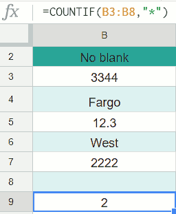
Column B has, we’re not going to count the header, two cells with text in it and we got that by using the function COUNTIF. The syntax is =COUNTIF(B3:B8,"*") which counts any cells with characters in it. That’s what this wildcard character * means. You use the quotes to let Google Sheets know that it’s a character and the asterisks is a special character that means anything. So, this is counting cells if there’s anything. However, if you take a looked at the next column in the live spreadsheet or in the next image, you can see the value is 3 and not 2.
Watch the video
Dealing with empty spaces
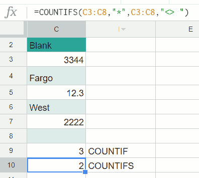
COUNTIF unless empty space
If you’re using the simple COUNTIF formula and getting a higher number than it should be, you may have some cells that have a space in them. They have a value, but you can’t see it. In the image above, C8 has one empty space in it. If you want to count that then you’re done here. The COUNTIF function with the asterisk is all you need. But, if you don’t want to count empty spaces, then you can use the function that we have in C10, =COUNTIFS(C3:C8,"*",C3:C8,"<> "). COUNTIFS means count if but plural so there are multiple criteria to consider. The first part is the same COUNTIF if there’s any character. But, we are saying also if it’s not just a blank space. When you put these two together in this compound COUNTIFS function, it doesn’t count the blank space that’s in cell C8.
So, column B is the easy way if you don’t have blank spaces. But, if you do have spaces, you want to use COUNTIFS. Keep in mind though, that the COUNTIFS above is just skipping cells with one space, you will have to extend the function if you have cells with multiple spaces.
Last minute reminders
A few things to remember are if the cell has a true/false value that’s not going to count. If the cell starts with a single quote, no matter what it has, that will count. Numbers are not counted by this function unless they’re entered as text. So another way to enter a number as text is to do the single quote and then type 333. That’s going to be counted because it’s not really a number, it’s the word if you will 333. I hope that’s helpful. Thanks!
Live examples in Sheets
Go to this spreadsheet for examples of COUNT that you can study and use anywhere you would like.