To sort your spreadsheet data in a powerful and organized way, we can add Pivot Tables to isolate specific data, then Slicers to further sort those tables. These filters can sort data in a different way than the built-in pivot table filters and provide additional options for your data sets.
For this example, we will keep the source sheet as is and display the filtered list. The starting data is a typical spreadsheet we will utilize in two pivot tables.

Create your Pivot Table
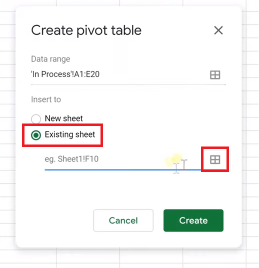
To create the first Pivot Table, go to Data, then Pivot Table.

We will use the source as the entire table, including headers. We will show the sales by item and an additional Pivot Table to sort by item and date. Use the OmniPivot add-on to use more than one Data range.

Select “Existing Sheet” and drop the table into G2 by clicking the box to the right, then selecting G2.

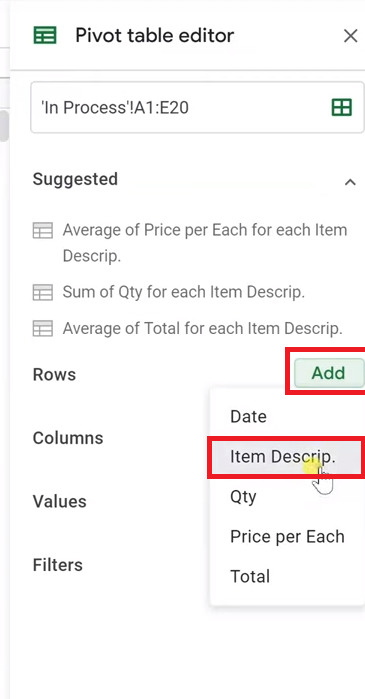
We’ll sort this by the sales quantity by item description. Next to Rows in the Pivot Table Editor, click Add, and select Item Description.

The Value will be “Quantity Sold.” We want this to be summed, so we will leave this drop-down with the SUM value. This creates a simple table that sums the sales by item description.

Create Another Pivot Table
To create the second Pivot Table, once again select Data then Pivot Table. We’ll use this table as a source and put this in G13. We’ll leave space because pivot tables expand and contract depending on what you do with them.

First, we’ll add a row for the dates using the same method above, then right-click and group the dates. Go to “Create Pivot Date Group” and click “Month” for this example. We’ll do quantity again as the Value to populate the total sales for the items.

This means we’ll need to add items to this second Pivot Table, so we’ll drop in another row by clicking the Add button next to Row, and selecting Item Description.

These two different tables are showing the same data in different ways – one by item description and one by item description and date.
Filter – First Method
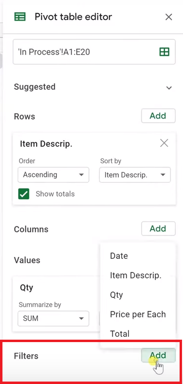
The first way to filter these Pivot Tables is to create normal filters that will act on both of these pivot tables as long as they are in the same sheet and working on the same data. Left-click on the Pivot Table, then go to the bottom of the editor to add a filter – let’s say to filter Item Description.

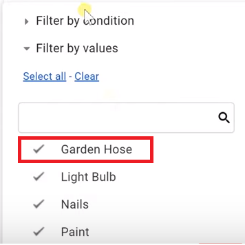
If you left-click on the status, you can either filter by condition or by values (which will be the same in the slicer). We’re going to take “garden hose” out.

Filters are specific to one pivot table. You won’t see this being filtered unless you look at the options in the editor. If we remove the filter, Garden Hoses will come back to the table. This means that no one will be able to see that this data is being filtered unless they look at the editor. This also only applies to one Pivot Table.

New Filter Option – Slicers
Instead of filters, we’re going to use Slicers and see how they operate differently. Go to Data then Slicer.

Now it’s asking for the data range. Click the original table, not the pivot table, for the data range. We’re going to slice the source data.

Drag the slicer over to the right. Since we’ve already selected the range, it automatically populates in the Slicer options. We’re going to skip the column for now, and we’re going to make sure that the checkbox is selected so that it applies to Pivot Tables.

In addition, you can further customize the slicer by choosing different colors, fonts, etc. Let’s leave it the way it is.

Let’s filter by item description. We can only do one column right now – if we need more, we’ll need to make additional Slicers.

The first thing we’re going to notice is that the Slicer is already here for everyone to see. There are the same options to filter by conditions and values when you click it. We’re going to do the same thing again and filter out Garden Hose. Start by clicking the Filter icon on the left.

Add Another Slicer
The data still exists but is hidden. If we want to filter by date, we will have to add an additional Slicer. All the Slicers on one sheet have to work with the same ranges. Additionally, they are sheet specific, so they will only filter the data on the original sheet.
The changes we have been making will only work in our user profile with our sheet, so if you want these settings to apply to additional users, you need to edit the slicer and pick “Set Current Filters as Default” – that way they will see the same filters that you have.

Let’s continue filtering by date. We’re going to select date once again, and “Filter by Condition.” We only want it if it’s after August 1st, 2019. This table only has July values on it.


Before I click “okay” we can see that this table has July values in it. When we update it, it will only have august.

Now the sheet has both Slicer filters applied.

One thought on “Google Sheets – Use Slicers to Filter a Pivot Table on the Fly”
Comments are closed.