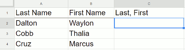
If you’re using Google Sheets and you have two columns of data that you want to join together, there are a few easy steps that we can walk through to get this done. In the following example, we have people’s first names and last names. This is a fairly common scenario. We are going to join them together and put a comma in between them.
First name and last name, not yet combined
The Formula
Place your cursor to the right of the two cells that you want to combine. In this example, it would be cell C2. As always, when you are entering a formula in Google Sheets, start out with an equal sign, and then indicate what you want to have joined together using this formula – =A2&", "&B2.
After entering this formula, you should see the first combined name.
Video Explanation
To copy this all the way down, place your cursor in the lower right hand corner of the rectangle. There’ll be a small solid blue square and your cursor will turn into a blue plus sign. Double-click the blue box and it copies the formula all the way down.
The Result
First name and last name, and combined
Now, all of your names should be combined into one column, viola!
If you’re using Google Sheets and you have two separate columns of data in which you’re looking for matches, there’s a pretty easy way to highlight the matched items. You can also do it the other way around and highlight items that don’t match. You’re typically doing this because your lists are long and you can’t do it visually. However, for this example the lists are purposely small so it’s easy to see.
Matches between two columns are highlighted
Conditional Formatting
We’re going to do it through Conditional Formatting. Go to your menu, then to Format, and select Conditional formatting. The Conditional formatting menu options will pop up on the right-hand side and there’s everything you need right here.
If you want to learn more about the complex subject of conditional formatting, I have created a course about it over at Datacamp. This is an affiliate link and if you use it to make a purchase I will receive a portion of the proceeds. Thank you for supporting my channel!
Menu option for conditional formatting
Rules for conditional formatting
First, apply the conditional formatting to the range which, in this shared spreadsheet (which is also embedded near the end of this page), is C1 to C10. Note that the range is different in the video but the process is the same. You can select the range with your mouse or type it in as C1:C10.
At first, the range should be highlighted because it is set to highlight if it’s not empty. Change this to a custom formula, which is at the bottom. Click on Custom formula is and then it gives you a box that’s waiting for the formula.
Custom formula
You are going to be typing in a formula just like you’re typing into a spreadsheet cell. One of the differences though is now Google Sheets is not going to help you. Once you start typing the function, no helper text will pop up to explain the function. If you want help, type the formula into a cell in the spreadsheet and it’ll help you build it. Then, you can paste it into the custom formula box.
Video explanation
MATCH formula
You want to use a function called MATCH. MATCH is going to look at each cell in the range and check to see if it exists in the other range that you specify. The first parameter that you want, it’s going to do this one cell at a time, is C1. Now type a comma and Sheets will be looking for the range that you want to try to look up C1 in to see if it’s a duplicate. You don’t want this range to shift down every time it evaluates a cell on the right., so use dollar signs before the row numbers to fix the range as such A$1:A$7.
Next, your spreadsheet wants to know if this is going to be an exact match. Enter a 0 (zero) for yes so if it finds exactly Yellow. Now close it off with the parentheses. Your code should look like this:
=MATCH(C1,A$1:A$7,0)
The box that contains this function should have changed from red to blue meaning that the function is now a valid function. It should be working after the box turns blue. You can see it highlighted the color red in green because red is on the list on the left but it didn’t highlight orange because orange isn’t in that list. If you click done, you’ve highlighted everything that exists in the other list.
=ISNA(MATCH(C1,A$1:A$7,0))
If you want to do this the opposite way, and highlight the items in this list that aren’t in the list on the left, wrap your formula in the function called ISNA. The ISNA function is saying – look, if the MATCH function doesn’t work, highlight it. Not if it does work. After the ISNA, put a parenthesis and then go to the very end and close it with the parenthesis.
View of Sheet with ISNA applied
Live examples in Sheets
Go to this spreadsheet for examples of comparing two lists that you can study and use anywhere you would like.
Using a plugin
As an alternative to the options above, you may want a plugin to do the heavy lifting for you. I like to use a plugin called Power Tools. This will give you a menu option with, among other things, several options to deal with duplicates. You can use the plugin to combine or remove duplicated rows.
Dedupe and Compare Menu
Conclusion
After following this tutorial, you should be able to highlight matches or differences between two columns. If you have any questions, feel free to leave a comment below.
Disclosure: This is an independently owned website that sometimes receives compensation from the company's mentioned products. Prolific Oaktree tests each product, and any opinions expressed here are our own.
If you want to track your employees’ time, there is an easy way to do it using Google Sheets that does not involve complicated formulas or macros. This technique will also have the ability to calculate an overnight shift. The linked file that can be copied into your own Drive and used as a template.
Data validation
One of the most difficult things when working with dates and time in Sheets is getting them in the cells correctly. A protection against that, data validation, can be used to reject invalid inputs.
Click on the Data menu option and then Data Validation.
Menu option for Data validation
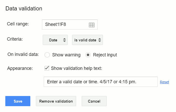
Once the Data validation window pops up, complete it with the parameters in the following pictures including choosing Date from the criteria drop-down box and rejecting invalid input with a message.
Choose date and is valid date
This will set data validation to show the message “Enter a valid date or time” if an invalid date is entered. Times are covered under the date formatting as card card-body bg-light so this data validation is also going to work if it’s a time. Now, if a user enters a date or time that Sheets doesn’t recognize as such, they will get an error message letting them know. There are several different ways to enter a date using a valid format, but there’s infinitely more ways to screw it up. You could do 2-20-18. You could type out February. But, as long as it’s valid, this timesheet will accept it.
The same thing is going to happen with time. If it’s 5:43 and the person types 5 43 in hits enter, it’s not going to work. You have to have a number, a colon, and a number. If you want seconds, do another colon and two digits after that such as 5:43:22.
The formula
Once the validation of the dates and times is set up correctly, the spreadsheet is ready for a start day and time and an end day and time. This formula is going to calculate the hours. So this formula is going to look a little complicated at first, but it’s really not too bad.
As seen in the shared sheet, this formula takes the row it is on and subtracts it from the row above it. To do arithmetic with these dates and times, Sheets has to convert them into a value first. That is what the DATEVALUE and TIMEVALUE functions are doing. The result will be a fraction of a day so multiply that by 24 and that gives you the number of hours worked. Every other row, you want to put in this formula.
If this person takes breaks, just repeat the same formula. If you want to make this longer, just copy and paste it down as many times as you want.
After following this tutorial, you should be able to create a time sheet to track the hours of your empoyees. If you have any questions, feel free to leave a comment below.
Live examples in Sheets
Go to this spreadsheet for examples of the time sheet that you can study and use anywhere you would like.
If you’re using Google sheets and you want to count the number of cells in a range that have text in them, as in text and not a number value, there’s a relatively easy way to do it. But, there are some hiccups with it and so we’re going to go through the easy way and a way which is a little bit more complicated but is more accurate. This tutorial will show you why each one works and which to use.
COUNTIF any text
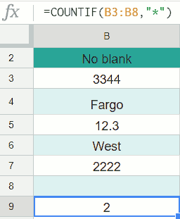
Column B has, we’re not going to count the header, two cells with text in it and we got that by using the function COUNTIF. The syntax is =COUNTIF(B3:B8,"*") which counts any cells with characters in it. That’s what this wildcard character * means. You use the quotes to let Google Sheets know that it’s a character and the asterisks is a special character that means anything. So, this is counting cells if there’s anything. However, if you take a looked at the next column in the live spreadsheet or in the next image, you can see the value is 3 and not 2.
Watch the video
Dealing with empty spaces
COUNTIF unless empty space
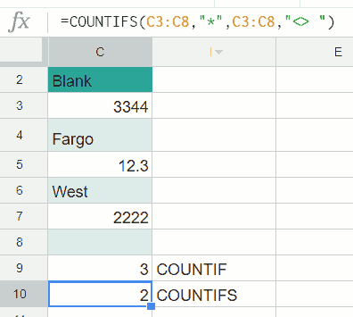
If you’re using the simple COUNTIF formula and getting a higher number than it should be, you may have some cells that have a space in them. They have a value, but you can’t see it. In the image above, C8 has one empty space in it. If you want to count that then you’re done here. The COUNTIF function with the asterisk is all you need. But, if you don’t want to count empty spaces, then you can use the function that we have in C10, =COUNTIFS(C3:C8,"*",C3:C8,"<> "). COUNTIFS means count if but plural so there are multiple criteria to consider. The first part is the same COUNTIF if there’s any character. But, we are saying also if it’s not just a blank space. When you put these two together in this compound COUNTIFS function, it doesn’t count the blank space that’s in cell C8.
So, column B is the easy way if you don’t have blank spaces. But, if you do have spaces, you want to use COUNTIFS. Keep in mind though, that the COUNTIFS above is just skipping cells with one space, you will have to extend the function if you have cells with multiple spaces.
Last minute reminders
A few things to remember are if the cell has a true/false value that’s not going to count. If the cell starts with a single quote, no matter what it has, that will count. Numbers are not counted by this function unless they’re entered as text. So another way to enter a number as text is to do the single quote and then type 333. That’s going to be counted because it’s not really a number, it’s the word if you will 333. I hope that’s helpful. Thanks!
Live examples in Sheets
Go to this spreadsheet for examples of COUNT that you can study and use anywhere you would like.
In this first set of data in the image above and also in this linked spreadsheet, we will be counting any cells that contain the word “Yellow” and only that word. To count the occurrences of the word yellow in the range B2 to B9 you can use the count COUNTIF function as such: =COUNTIF(B2:B9,"yellow"). It performs a conditional count. In this case, only if the cell or ranges of cells is equal to Yellow. Yellow is not case-sensitive so this is going to pick up three instances even though B7 is not capitalized. If the COUNTIF technique is doing everything you need, then you’re done and there is no need to try anything more involved.
Looking for a word occurring anywhere a cell
COUNTIF with wildcard
Looking at this second set of data, things will get a little bit more complicated. We are looking for a certain word that occurs anywhere in any of these cells. First, you want to use COUNTIF again and give it a range =COUNTIF(C2:C9, "*Yellow*"). For this example, the range will be C2 to C9. If it has the word yellow and anything before which is what the asterisk means, and anything after it which is the second asterisk, then it should be counted. It just has to have yellow in some part of it. Anything can be nothing so it can start or end with yellow too. This function is also counting 3 because of the yellow plane, the yellow car, and the little yellow boat.
Case-Sensitivity
The COUNTIF function is not case-sensitive. To count cells with specific capitalization, follow the second example in this tutorial.
Using a plugin
As an alternative to the options above, you may want a plugin to do the heavy lifting for you. I like to use a plugin called Power Tools. This will give you a menu option with, among other things, advanced Find and Replace features. This will give you a list of all the occurrences of a word in your spreadsheet, but it won’t give you a count of them. Depending on the size of the spreadsheet, this may be the preferable option.
Find and Replace Menu
I hope that was helpful and now you know the formula for counting any occurrences of any word that you’re looking for.
Live examples in Sheets
Go to this spreadsheet for examples counting specific text that you can study and use anywhere you would like.
Disclosure: This is an independently owned website that sometimes receives compensation from the company's mentioned products. Prolific Oaktree tests each product, and any opinions expressed here are our own.