If you are working on a large table of data in Google Sheets, often it is helpful to be able to see and edit more than one area of the spreadsheet at a time. This is not available from the menus in Sheets and is one of the few ways in which Excel is superior to Sheets. There is the option to Freeze rows or columns, but the frozen section of the spreadsheet will not independently move and therefore the Freeze option is limited to applications such as freezing headers at the top or side of a spreadsheet. Further, if you headers are half way down the spreadsheet, the Freeze option will not do you any good.
The solution
If you are working on a mobile device you may be out of luck, but if you are accessing Sheets through a browser, there is a great work around that will allow you to see the same spreadsheet in two or more different windows. You can even spread these views over multiple monitors which you cannot do in Excel without some pretty nasty workarounds.
Watch the video
If you are using the Chrome browser, do the following:
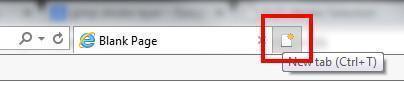
First, be sure to have your spreadsheet open in your browser. Then, open a new browser tab by pressing “t” while holding down the control button (ctl+t) or clicking the shape to the right of your open tab.
Once you have a new tab open, the first thing you do is open the same spreadsheet again in this new window. Now, you have the spreadsheet open in two places. You can edit it in either window. Click and hold your left mouse button on the middle of the new tab, where the title of the page is, and pull the tab away from the browse. In browsers other than chrome, you may have have to open another browser window. This creates a new window with a separate instance of Chrome (or other browser) but keeps the spreadsheet inside of it.
If you want more windows, just repeat the same process. To rearrange the windows, you can use the Windows key. Hold the Windows key down and press the left arrow to have the window fill up the left half of the screen and the right arrow for the right half. You also can resize the windows the more traditional way with your mouse. If you have multiple monitors, you can spread these windows across them.
Using multiple tabs in other browsers
Update: Thanks to ADTC in the comments below for this tip. If you’re using Chrome, you can just right-click on the tab that you’re using and choose duplicate.
If you are using Google Sheets, you may be having some trouble finding how to insert a line. Once you have figured out how to insert it, getting it to be straight can be frustrating. Follow these easy steps to get it done.
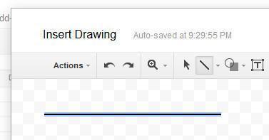
Go to Insert, then Drawing.
From here, choose Line.
Now, here’s where the real trick comes in. If you want to draw a line, go ahead. But, if you want to draw a straight line, hold down the shift key while you draw! There it is, a straight line.
If you are using Google Slides, you may be having some trouble finding how to insert a line. Once you have figured out how to insert it, getting it to be also straight can be frustrating. Follow these easy steps to get it done.
Go to menu bar and select line.
Line option on the main menu
Watch the video
Now, here’s where the real trick comes in. If you want to draw a line, go ahead. But, if you want to draw a straight line, hold down the shift key while you draw! There it is, a straight line.
5 Ways to alter the orientation of the text in a cell
Spoiler altert – all of them are workarounds!
As of late February, 2017, the ability to rotate text is native to Google Sheets. The option is the slanted A on the main menu to the right of text wrapping.
Use a text box then rotate it
Text boxes are inserted using the drawing menu with Insert-> Drawing -> Text Box. As can be seen in the picture, they do not reside in a cell, but rather they sit on top of them. This is why the text box will not affect your row height. Once the text box is created, it can be rotated as much as you would like. After rotating it, you can then move the text box to wherever you would like it.
Video explanation
Skinny column with wrapped text
You can also achieve vertical text by typing the text in the cell normally. Then, you shrink the width of the column to a little more than one character wide. Next, you apply word wrap by selection Text Wrapping (on the menu bar) then Wrap. One disadvantage of this method (and all of the remaining methods) is that it alters the height of the row in which it is placed. Also, the technique requires that the column is skinny and therefore it will limit the way in which other content can be viewed if it is in the same column. Depending on how you are using the vertical text, this may or may not be a problem.
Array formula
Just put the text that you want into this crazy formula. Remember to type it in both places.
=ARRAYFORMULA(CONCATENATE((MID( "Text to become vertical"; ROW(INDIRECT("YY1:YY"&LEN( "Text to become vertical" ))); 1)&CHAR(10))))
How does it work? Who cares! Just use this method if you find it easier.
Regular Expression
Similar to the array formula, just a crazy formula into which you can insert your text.
=REGEXREPLACE( "Text", "(.)", "$1"&CHAR(10) )
I would say that you should use this formula as opposed to the Array formula simply because it is shorter and you only need to type the text once.
Control Enter
If you hold down the control key then press enter after a character, you will get a new line within that cell. Therefore, to enter vertical text, just type control enter after every letter. In my humble opinion, this is probably the cleanest solution until there is a true option is Sheets to rotate text in a cell. It does not require the column to be a certain width nor do you need a long formula.
Follow image below for the live Google doc with this data
There are several free options for online spreadsheet creating these days. The two most popular free options are Google’s Sheets and Apple’s Numbers, for which you need a free iCloud account. These programs can be used on a wide range of devices. Most of the screen shots below are from an iPad. Once you have chosen your program and created an account –
Start with a blank spreadsheet
Create a header row
Video explanation
Type the following values in cells A1 through A7.
Date – The date you made the deposit, wrote the check, etc. Note that this date does not always correspond to the date on which the transaction is posted to your bank account. This time lag creates the need to reconcile the account monthly. See how to do that in this post.
Check Number – This field is perhaps a bit outdated. 15 years ago, most payments coming out of a checking account would have been from paper checks. Presently, many are ACH’s or payments made directly from a bank’s website. However, this field can still be useful. You can use it simply for the checks that you still write, or you can be more creative with it and put confirmation numbers in it for online payments.
Cleared – This is the column that you use when you do your monthly reconciliation. You put an asterisk (or any other symbol) here when you see that the deposit or payment cleared the bank in the month in which you are performing your reconciliation.
Description – At the least, use this field to specify the payee for amounts going out and the payor for deposits coming in. Since it is a spreadsheet, and not a paper ledger, you can type as much as you want here. Take advantage of this. No one ever regrets having too much documentation. If you have a deposit from multiple people, write out all of their names and the amounts. Later, when you are trying to figure out if Mrs. So and So paid you, you can use search the spreadsheet (Ctl + F as a shortcut) and quickly find out.
Debit – Use this column for your payments out of the account. Admittedly, this is the opposite of what you would do if you were an accountant for a company using the double entry method. However, I chose to make my register this way because your bank calls payments debits and deposits credits so I find this less confusing.
Credit – Enter deposit amounts in this column
Balance – This will be the running total of your credits less your debits. Now, keeping this number large is your job!
Record your first entry
This is probably a deposit for an opening balance. The amount for this would go in the credit column. The formula for the Balance column is different on the first line. Note that formulas are started with the “=” sign. This is what tells a spreadsheet that your are entering a formula and it should display the result. The formula is simply:
=F2
This will display the value that you entered in the credit column. Note that the screenshots are from an iPad. Depending on what device you are using, the screen may look a bit different.
Use styles to display dollars and cents
As shown in the image above, numbers do not always display the way that you would like them to. When working with currency, it is typically helpful to see dollars and cents even when your amounts are in whole dollars. When you have a larger amount of transactions, having all of the number amounts display the same makes them easier to look through. If you don’t format these numbers, 1,000.01 will look significantly larger than 1000 when you are glancing at it. If they both display as 1,000.00 and 1,000.01, you will be able to tell the difference faster. Also, a comma can be helpful when the numbers get larger but a dollar sign can be redundant. If you are using Google Sheets, use the following steps to style the numbers.
First, select all of the columns to which you would like to apply the styles. If you only select certain cells, you will have to redo the styles when you add more rows.
Click on formatting and choose cell formatting then number format.
That should do it. Now your amounts will be easier to scan through.
Entering the next transaction
Now enter your next transaction in row 3. Whether this is a debit or a credit, this next formula will corrrectly capture it and add or subtract it from your balance. Note that the formula starts with an equals sign which is the universal technique for telling a spreadsheet that you are entering a formula instead of a value.
=G2-E3+E4
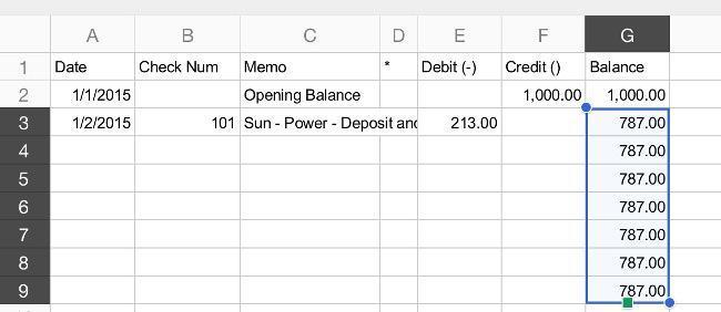
This formula is the only one that you will need from this point forward. You should copy this formula down this column for thirty lines or so, enough to give you some room to work without copying it again. Depending on what device you are using, there are multiple ways to copy a formula down. The most intuitive is copy and past the same way that you would with any other program. The easiest is to move the cursor to the lower right corner of the cell, until it changes to a different icon, then drag the outline down as far as you would like. When you copy formulas, the spreadsheet is smart enough to increment the cell references so they are always pointing at the appropriate line. If you are using Sheets on a tablet, select the rows you want to copy. Make sure you get a green dot on the rectangle that surrounds your selection as shown below. This image is shown after the green dot appeared and the user dragged it down with their finger.
When you are entering your descriptions, make them as long as you need to. You can search through your descriptions to find things later so pack them with the keywords that you think will be helpful. The next cell will just overlap the data but not erase it. See the highlighted portion below illustrating how the text is overlapped but is still saved and searchable.
See an example of this checkbook here as a shared Google Sheet. This spreadsheet is configured so that anyone can view it but not edit it.
Live examples in Sheets
Go to this spreadsheet for examples that you can study and use anywhere you would like.
You know have a simple, useful check register that you can access from anywhere that you have a web connection as Google Sheets and Apple Numbers can be used on mobile devices as well as laptops and desktops.


 Create a header row