Insert checkbox menu option

Google Sheets – Create an Interactive Task List

This tutorial will show you how to create an interactive to-do list in Google Sheets including automatic strikethroughs when you mark tasks complete with a checkmark.

Insert Checkboxes

Insert checkbox menu option
Insert-> Checkbox

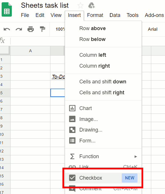
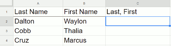
As shown in the image above, the core functionality of this list will be driven by checkboxes. You can enter them into your spreadsheet by going to the Insert menu and choosing Checkbox. Insert one and then copy and paste it down until you have as many as you want. Add your tasks in the column to the right of the checkboxes.

Conditional Formatting

Now, if you’re like me, when you’re done with the task, you’d love to be able to check it off and get a little strikethrough, right? You can feel like you’re accomplishing something. The strike through will come from using the conditional formatting feature.

Conditional formatting
Conditional formatting menu option

After selecting Conditional formatting, a Conditional formatting rules box will appear on the right. Look closely at the picture below. For the range, we have specified C5:C which will select everything in column C from row 5 and below, assuming that is where you have placed your list of tasks. Once you move out of this input field, you should see that everything in column C starting a row 5 and down to the end of where you have things typed is highlighted.

If you want to learn more about the complex subject of conditional formatting, I have created a course about it over at Datacamp. This is an affiliate link and if you use it to make a purchase I will receive a portion of the proceeds. Thank you for supporting my channel!

Conditional formatting rules

Watch the Video

Custom formula

Right now, it’s just applying formatting as Cell is not empty because that’s the default choice. Change that by going to the drop down menu below Format cells if… and choosing Custom formula is. Now this box is waiting for a custom formula. Left-click into it to put the cursor in it. Whenever you’re typing a formula, even if it’s in here, you start it with an equals sign. Type the formula =B5=TRUE. Make sure you don’t use the period at the end. When a checkbox is checked, it changes the value of the cell from FALSE to TRUE. This formula will check for the TRUE state.

If the value is true, we will apply Custom Formatting style. Choose a style to make strike it through and make the background gray so it looks like it’s going away.

If you want to add something else at the bottom, you won’t have to redo this rule because that formatting contains the entire column after C5.

Completed Task List

Finished task list

Pretty easy to put together. Really satisfying to use. Have some fun with it, and let us know how it turns out.

 Live examples in Sheets

Go tothis spreadsheet for examples of adding and subtracting days, months, or years that you can study and use anywhere you would like.
Cells with data to be combined

Combine Cell Contents from Two Different Columns in Google Sheets

Separate Cells Needing to Be Joined

If you’re using Google Sheets and you have two columns of data that you want to join together, there are a few easy steps that we can walk through to get this done. In the following example, we have people’s first names and last names. This is a fairly common scenario. We are going to join them together and put a comma in between them.

Cells with data to be combined
First name and last name, not yet combined

The Formula

Place your cursor to the right of the two cells that you want to combine. In this example, it would be cell C2. As always, when you are entering a formula in Google Sheets, start out with an equal sign, and then indicate what you want to have joined together using this formula – =A2&", "&B2.

After entering this formula, you should see the first combined name.

Video Explanation

To copy this all the way down, place your cursor in the lower right hand corner of the rectangle. There’ll be a small solid blue square and your cursor will turn into a blue plus sign. Double-click the blue box and it copies the formula all the way down.

The Result

Cells with data to be combined
First name and last name, and combined

Now, all of your names should be combined into one column, viola!

Live Google Sheet with This Data

docs share icon

Google Maps What's Here

How to Find the Plus Code for Any Location

If you want to find a Plus Code for a certain location, it is not that easy. At this point, you can’t do it on Google Maps. When you left-click on an area and choose What’s here?, it will give you latitude and longitude but Maps does not give you the Plus Code.

Google Maps What's Here
Place info on Google Maps
Latitude and Longitute
Latitude and longitude

However, what you can do is, you can go to plus.codes and use the Find your code option.

Plus Codes Website
plus.codes

Zoom in or out until the area that you want fills the screen. A Plus Code designates an area in the shape of a rectangle. It’s not a point like latitude and longitude. You can take advantage of that by zooming in and out until you get to the size of an area that you want. After you have the right area, go to the menu and choose the option to see the Grid.

Menu on plus codes site
Map menu
Grip option on menu
Option to show grid

Video explanation

After choosing the option to show the grid, you will see the rectangles that are available to you. In this case, the area labeled 86FVCF fits Hocking Hills State Park which is the area that I am looking for. 86FVCF is the first part of the full Plus Code that you will see later in this article.

Seeing 86FV in grid
Grid shown over map

There is also a shortened code available at the bottom of the screen. CFG7+JP, works for anyone that lives close to the park. It’s a shortened, partial version of the code. CFG7+JP does not contain the beginning 86FV portion of the 86FVCF code, so it works when you are already relatively close to the area.

Plus code
Shortened Plus Code

On the left side of the plus.codes screen, you will see the full Plus Code and the shortened Plus Code that can be used for local navigation. If you want the entire Plus Code, which is probably the best practice if you are copy/pasting, go to the left of the screen and copy it. This is your full Plus Code. It’s not case-sensitive, but since we’re copy and pasting it in, it doesn’t matter.

Codes
Left side of plus.codes showing full and shortened Plus Codes

Go back to your mapping program, which is Google Maps in this case, and enter this Open Location Code into the search bar. Google Maps will go to the area that corresponds to the Plus Code and drop a pin in the middle of it. Maps shows you the latitude and longitude of the center of the Plus Code but it will not show the grid with the codes on it.

Plus code in Google Maps
Google Maps searching for Plus Code
Hocking Hills on Map
After searching for Plus Code

Now you know how to find your Plus Code using plus.codes with the grid feature turned on and you can take that Plus Code and enter it into Google Maps, you know how to find and use a Plus Code. I hope that was helpful!

Two columns with matches highlighted

Google Sheets – Compare two lists for matches or differences

If you’re using Google Sheets and you have two separate columns of data in which you’re looking for matches, there’s a pretty easy way to highlight the matched items. You can also do it the other way around and highlight items that don’t match. You’re typically doing this because your lists are long and you can’t do it visually. However, for this example the lists are purposely small so it’s easy to see.

Two columns with matches highlighted
Matches between two columns are highlighted

Conditional Formatting

We’re going to do it through Conditional Formatting. Go to your menu, then to Format, and select Conditional formatting. The Conditional formatting menu options will pop up on the right-hand side and there’s everything you need right here.

If you want to learn more about the complex subject of conditional formatting, I have created a course about it over at Datacamp. This is an affiliate link and if you use it to make a purchase I will receive a portion of the proceeds. Thank you for supporting my channel!

Conditional formatting menu option
Menu option for conditional formatting
Rules for conditional formatting

First, apply the conditional formatting to the range which, in this shared spreadsheet (which is also embedded near the end of this page), is C1 to C10. Note that the range is different in the video but the process is the same. You can select the range with your mouse or type it in as C1:C10.

At first, the range should be highlighted because it is set to highlight if it’s not empty. Change this to a custom formula, which is at the bottom. Click on Custom formula is and then it gives you a box that’s waiting for the formula.

Custom formula
Custom formula

You are going to be typing in a formula just like you’re typing into a spreadsheet cell. One of the differences though is now Google Sheets is not going to help you. Once you start typing the function, no helper text will pop up to explain the function. If you want help, type the formula into a cell in the spreadsheet and it’ll help you build it. Then, you can paste it into the custom formula box.

Video explanation

MATCH formula

You want to use a function called MATCH. MATCH is going to look at each cell in the range and check to see if it exists in the other range that you specify. The first parameter that you want, it’s going to do this one cell at a time, is C1. Now type a comma and Sheets will be looking for the range that you want to try to look up C1 in to see if it’s a duplicate. You don’t want this range to shift down every time it evaluates a cell on the right., so use dollar signs before the row numbers to fix the range as such A$1:A$7.

Next, your spreadsheet wants to know if this is going to be an exact match. Enter a 0 (zero) for yes so if it finds exactly Yellow. Now close it off with the parentheses. Your code should look like this:

=MATCH(C1,A$1:A$7,0)

The box that contains this function should have changed from red to blue meaning that the function is now a valid function. It should be working after the box turns blue. You can see it highlighted the color red in green because red is on the list on the left but it didn’t highlight orange because orange isn’t in that list. If you click done, you’ve highlighted everything that exists in the other list.

=ISNA(MATCH(C1,A$1:A$7,0))

If you want to do this the opposite way, and highlight the items in this list that aren’t in the list on the left, wrap your formula in the function called ISNA. The ISNA function is saying – look, if the MATCH function doesn’t work, highlight it. Not if it does work. After the ISNA, put a parenthesis and then go to the very end and close it with the parenthesis.

View of Sheet with ISNA applied

 Live examples in Sheets

Go to this spreadsheet for examples of comparing two lists that you can study and use anywhere you would like.

Using a plugin

As an alternative to the options above, you may want a plugin to do the heavy lifting for you. I like to use a plugin called Power Tools. This will give you a menu option with, among other things, several options to deal with duplicates. You can use the plugin to combine or remove duplicated rows.

Dedupe and Compare Menu

Conclusion

After following this tutorial, you should be able to highlight matches or differences between two columns. If you have any questions, feel free to leave a comment below.

Disclosure: This is an independently owned website that sometimes receives compensation from the company's mentioned products. Prolific Oaktree tests each product, and any opinions expressed here are our own.

Title of Sway

Embed a Live Word Document into a Microsoft Sway Presentation

If you’re using Microsoft’s Sway and you want to insert a Word document, there’s just a couple easy steps to do it.

Title of Sway
The title of your Sway

Create a new Sway and give it a title. I’ve called this one Embedding a Word Document.

Media group
Choose the media group

Next, click the plus sign to add more content. Choose the Media group then click the Embed option.

Embed
Choose the embed option

Video explanation

https://www.youtube.com/watch?v=9Cnb9eqSvnA”

Create new Word document
Create a new Word Document
Upload Word document
Upload an existing Word document

Sway is now waiting for the embed code. You need to get the code from your Word document after you’ve uploaded it to OneDrive (or created it online to begin with). So, assuming you’ve uploaded your Word document, we’re going to step forward from that point. If you haven’t done that, you need to open up OneDrive and upload it.

Embed option in Word
Embed option in Word online

In the online Word document, go to Share and embed and the code is down here waiting for you. It’s all highlighted. Copy the embed code from your clipboard and go back to your Microsoft Sway. Go to the box waiting for your input, and paste the code.

Embed card with code
Sway card with embed code

You’ve embedded that Microsoft document. This is live. If you were to update this in Word, this document that’s showing here would be updated. You can also interact with this document to a certain extent with the icon lower right hand corner. You can download it or print it.

Sway with embedded document