-UPDATE- As of November 2016, their is a “Create a filter” option in the menus for Google Sheets on an iPad. You can find it by clicking the three vertically algined dots in the upper right hand corner of your spreadsheet. The tips below still apply to using the FILTER function, but it is not your only choice for filtering on an iPad now.
Most spreadsheet users are used to performing all of their functions through the menus with the click of a mouse. However, today’s mobile versions of these programs offer very few options through their menus. The FILTER function, much like the SORT function function, is one of those options that lost its coveted menu spot and has been relegated to the list of functions that must be typed in or found in the list of every function available in Sheets.
Before you enter your filter formula, you will want to select a cell that will be the upper left most cell for the filtered list. This function writes the data below and to the right of your starting point. Once you find the right cell, enter the command using the following syntax:
=FILTER(range, condition1, [condition2, ...])
In the formula above, FILTER is the name of the function, range is the table of data that you want to be filtered, and the conditions are how you want it to be sorted.
Video explanation
Find more information on the FILTER function at Sheetshelp.com.
One column
Let’s start with a simple example in the image below.  This is a small list of data. For whatever reason, you find the need to filter it. A list this small would be easier to just manipulate by deleting what you don’t want, but it is kept simple so the illustrations can get right to the point.

As you can see, the filter function creates a new list with just the data left that you specified. Be aware that the formula still remains in the cell in which you typed it. If you want to keep the data in this new list, you may want to consider copying it and pasting it as values. This will fix it in place even if the original data is changed.
Two columns
Next, let’s sort the table based on criteria that resides in neighboring cells. Select both rows and use the second field of the formula for the sort criteria of b1:b4=”b”.
=FILTER(al:b4,b1:b4="b")

This will create a new, filtered list with just the rows that contain the letter “b” in the second column. Again, the filtered data is still dynamic. If you change anything in the original list to be sorted, the new sorted list will also change.

Three columns
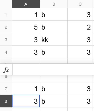
You can also filter a table based on multiple criteria. The picture below is showing an easy example of this. The formula works as an AND statement, meaning that both conditions need to be TRUE in order for the data to be output by the function.

The output of this formula is as follows. The function only kept the data that had a “b” in column B AND a 3 in column C.
Follow image below for the live Google Sheet with this data
![]()
Conclusion
Having the filter function available, even it is not in the menus, can be quite handy when you are working on a mobile device. For larger sets of data, the filter function can be faster and more accurate than sorting data manually. Enjoy and happy spreadsheeting to you all.