Let’s say you had several spreadsheets saved in Google Drive, and we wanted to combine them into one spreadsheet; how would we do this?
As explained in 📺this video, we can use formulas, but this gets tedious when dealing with a large number of sheets. Instead, we can use a Google Sheet add-on known as Power Tools.
The first thing to note is that the data must have matching headers. They don’t have to be in the same order across all spreadsheets, but they need to match. We can combine the data in a static way or make sure that it’s dynamic by auto-inserting the formulas.
In our case, we are going to combine three spreadsheets that contain lists of companies. Here’s a look at one of the sheets to better understand what we’re working with.
There are two other similar sheets – Australian companies & USA companies. Now let’s combine them.
Combining Static Spreadsheets
These are the steps to follow when combining the data is a one-time operation that doesn’t need to update when any of the sheets changes:
Launch Power Tools via Add-ons > Power Tools. (If you haven’t installed Power Tools yet, you can follow this link to install.
In the sidebar on the right, select “Merge & Combine.”
Select “Combine sheets” and click on “Add files from Drive” in the pop-up that appears.
Add all the sheets from which you would like to fetch data.
Make sure the boxes are next to the files and click “Next.”
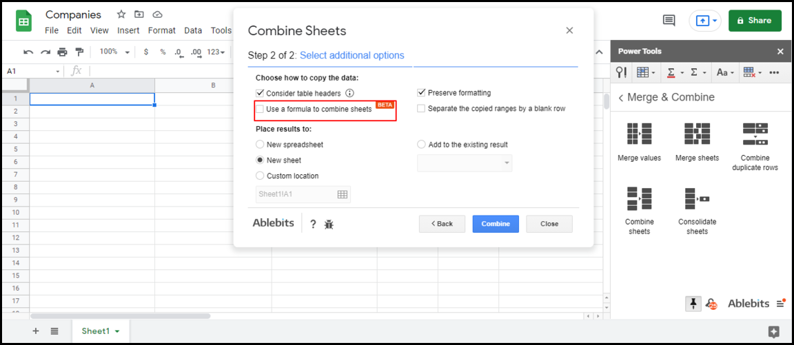
In the following pop-up that appears next, make sure that “Use a formula to combine sheets” is not checked. (This is because we are working with static data). Now click combine.
After a few seconds, a new sheet within the spreadsheet will appear with the combined data.
Combine Dynamic Spreadsheets
If we need the combined data to be dynamic, Power Tools can automatically insert the formulas we need. To do this, follow the steps we used in the previous example but, this time, make sure that the box labeled “Use a formula to combine sheets” is checked.
Upon combining, the sheet containing combined data will appear with errors since no user has granted permissions yet. (Remember we need to give access when using IMPORTRANGE). An extra sheet will appear, and we can then grant permissions there. That should correct the errors.
Since we’re using formulas, any changes to the source files will reflect on the combined sheet.
Disclosure: This is an independently owned website that sometimes receives compensation from the company's mentioned products. Prolific Oaktree tests each product, and any opinions expressed here are our own.
You may be looking for AutoSum in Google Sheets, but you won’t find it in the built-in menus.
AutoSum in Excel
Traditionally in Microsoft Excel, you would sum, multiply or divide values in a range by keying in the respective function and then specifying the range. You would add the total number of units In the following dataset by applying the formula, “=SUM(D2:D10)“.
However, as demonstrated in 📺this video, Excel provides a built-in intelligent function that automatically detects the range we wish to sum, known as AutoSum. If we place the cursor on cell D11 and click on AutoSum, Excel will figure out on its own that we intend to sum the range, D2:D10.
AutoSum in Google Sheets
Could we do the same in Google Sheets? Well, it’s not as impressive as in Excel. Instead of auto-detecting the range, Google Sheets merely inserts the specified function without the range.
We could solve this problem using a third-party add-on known as Power Tools.
After you install Power Tools, you can launch it via Add-ons > Power Tools > Start.
Now that we have the plugin installed, we can repeat the AutoSum operation we did in Excel. To achieve this, click on the cell that needs to add up the total. In our case, we want to get the Units total, so the cell is D11. Now that you have selected the units, head over to the sidebar and click on the AutoSum icon, Σ (not to be confused with the red-underlined Σ). Next, click on SUM in the drop-down that appears. After clicking, the total automatically appears in the cell we selected.
Things to note:
You can execute operations besides addition using the Power Tools add-on. The drop-down next to the icon provides a wide selection of functions to apply.
There’s an AutoSum by color function in Power Tools, which sums values based on background color and the text color. Find more on that here.
Disclosure: This is an independently owned website that sometimes receives compensation from the company's mentioned products. Prolific Oaktree tests each product, and any opinions expressed here are our own.
One of the great things about Google Sheets is that, when it comes to uploading images, you have the option to either upload images over cells (like you would with a text box), where they can be moved and resized freely, or upload the images inside the cells. However, you can upload files to a spreadsheet including images, PDFs, and Word docs to Spreadsheet.com and then some.
Not only can you upload images inside the cells, but you can also upload other file types such as PDFs, DOCX et cetera – a feature that is non-existent in both Google Sheets and Excel.
Uploading an Image over Cells in a Spreadsheet
Fist, to upload an image over a cell(s) in Spreadsheet.com, go to Insert > Image and select the desired image from the respective source:
Go to Insert > Image
It’s worth noting that Spreadsheet.com gives you the option to upload your image from various sources. Beyond uploading from your device, you can also upload from Google Drive, Box, OneDrive, or Dropbox:
Various upload sources are available
Uploading an Image inside a Spreadsheet Cell
To upload the image inside a cell, you have to first set the data type of the column to “attachment”. To do this simply click on the respective column header, click on the dropdown on the far right of the column header, click on “Edit data type…” and select “attachment”:
Go to the column header and click on “Edit data type…”
Set the type to “Attachment”
Notice that in the above pop-up, you have the option to make the cells of the column small, medium or large in order to comfortably accommodate the file types to be attached. There’s also the option to set the data type as strict which would prevent the entry of any other data type in the column save for the specified one.
Once the column data type is set as “attachment”, images can be added inside any cell in that column. To do this, simply click on the cell to add an image to, click on the “attach” icon:
Uploading other file types to your spreadsheet
As mentioned before, Spreadsheet.com edges out both Google Sheets and Excel considering the fact that you can upload files such as PDFs. But how do we upload other file types? Quite simply:
Set the column data type to “attachment” (as explained above)
Upload the desired file and it’s going to appear inside the cell.
A PDF file stored inside a cell would look like this:
Upon clicking the PDF, the document should open.
Note: Notably, you cannot add attachments to your primary column. You’d first have to de-select the primary column setting before you can add attachments to any cell in that column. Conversely, you cannot set a column to be a primary column if the specified data type is not “Standard”. You can read more about primary columns here.
You can have complete control over the look and feel of the numbers in your spreadsheet by using custom number formatting in Google Sheets. You can follow this example by starting with this template.
This article will walk you through the process of customizing the appearance of the numbers in your spreadsheet. Accordingly, it will teach you how to control your numbers’ visual presentation with currency signs, arrows, and more. Changing the look is called Custom Number Formatting. To have a comprehensive understanding of Custom Number Formatting, see this video from the Prolific Oaktree Youtube Channel.
Besides the default look, which presents your data in the black font color, you can infuse some level of creativity in your presentation by assigning different font colors to enhance the message of your presentation. For instance, you may want to present debits in red and credits in green.
Take a look at the image below.
Red and Green custom numbers
The data in red have a minus sign (-) before each, which indicates negative, hence, the use of red. On the other hand, the data in green is positive.
Changing the number formatting allows you to change the look, but the values of each cell will not change. It only gives it a different appearance through the color assigned to individual rows of data.
How To Custom Format Your Numbers in Google Sheets
The procedure is simple; locate your menu bar at the top of your spreadsheet and select Format>Number.
How to Format Numbers
After the number format menu appears, you will notice that there is a preset format for the display of your data. If that is what you want, you do not need to change anything. Just click on it, and you have your option activated.
However, if you want to give the data in each of the cells on your spreadsheet a custom look, you need to dig deeper. We will walk through how to get that done.
Customize the Look of Your Numbers in Google Sheets
The way your spreadsheet looks is up to you. Therefore, if you are not satisfied with the general format, this is how you can change it.
Highlight the columns with the numbers to be changed.
Click on Format on the menu bar.
Click on Number from the pop-down menu.
Check if there are pre-defined number formats for you to use (if not).
Click on More Formats.
Click on More Number Formats.
A dialogue box will pop up for you to choose the syntax:
Custom Number format
The syntaxes are below:
Input
0; -0; “-“; “not a number”
Output
Formats a positive number with 0
Formats a negative number with -0
Shows zero as a dash (“-“).
Shows a non-number as “not a number.” Anything in quotes in programming as a syntax remains as it is. The quotes signify that it is a string variable. The semicolon is to separate the columns.
If you intend to format a long number such as “$8,000,000,” you would use the “$#,##0.00” syntax. If you don’t intend to include the decimal points, enter “$#,##” and click the “Apply” option. Voila!
How To Insert Currency Before a Number in Google Sheets
To insert a currency sign before your number, the sign should precede the numbers in the syntax dialogue box such as we have below:
$* 0.00 – positive
$* – 0.00 – negative
The asterisk (*) gives space between the number and the currency sign. The two zeroes after the decimal force the display of tenths and hundredths.
How to Add Color to Custom Number Formatting
As earlier stated, you can give colors to your numbers for easy understanding.
To achieve customized color for your data, type the following syntax:
0[Green]; -0[Red]; ‘-‘[Black]
NOTE: The name of the color for each number format will come after each of the numbers in parentheses. Make sure you enclose the color for each cell in square brackets (Check the image below).
For the image below, the name for positive numbers is GREEN. Negative numbers are assigned RED. Zero will appear in BLACK.
Custom Color format
How to Insert Special Characters in Your Data in Google Sheets
Adding special characters to your presentation can make your Google Sheet easier to understand.
When using Google Sheets, often times you can find yourself wanting to pull data from one table into another. However, these two tables don’t always have the same types of data in the same order. As long as there is at least one value in common, you can use a few tricks to bring data from different tables together into one combined table.
We will go over how to do this using several relatively basic steps and ending with the super-useful VLOOKUP formula. VLOOKUP typically looks to the right (we’ll get there), but we can also trick the function and have it look to the left.
In September 2022, Google Released the XLOOKUP function. It is an easier to use and more flexible alternative to VLOOKUP.