When using Google Sheets, often times you can find yourself wanting to pull data from one table into another. However, these two tables don’t always have the same types of data in the same order. As long as there is at least one value in common, you can use a few tricks to bring data from different tables together into one combined table.
We will go over how to do this using several relatively basic steps and ending with the super-useful VLOOKUP formula. VLOOKUP typically looks to the right (we’ll get there), but we can also trick the function and have it look to the left.
In September 2022, Google Released the XLOOKUP function. It is an easier to use and more flexible alternative to VLOOKUP.
This post is written to accompany the YouTube video showing how to combine multiple tables of data in your Google Sheet without using the QUERY function.
Oftentimes, data that you want to analyze is spread across multiple sheets and multiple files. If you want to combine tables found on multiple worksheets and/or multiple worksheets, these four different techniques will help you join them together. Each technique results in different output. Choose the one that works best for you.
These methods are meant for data with like headers and data types.
Using UNIQUE
Four circumstances covered
Keep Original Order
Keep the order of the original data by stacking each list.
Sorted
Sort the resultant table by any column.
Duplicates removed
Remove any duplicate lines of data if you don’t want them in your sample.
No blank rows
Remove any blank rows from your new table.
Also, data from another file can be pulled into these formulas using the IMPORTRANGE function.
If you’re using Google Sheets and you have a list of amounts that you want to sum or count based on whether or not there are notes in the cells, there’s no built-in function to do it. However, there are a relatively easy set of steps to make your own functions to get it done. You’ll be able to COUNT based on cell notes and you’ll be able to SUM as well. Previously, we’ve made custom functions to COUNT or SUM by background color.
This video will walk you through the same steps described below.
Custom formulas in action
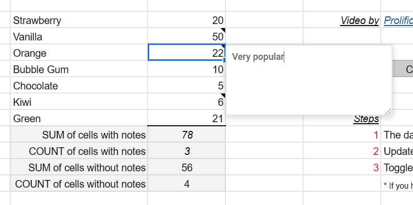
Cells being counted and summed by notes
SUM if there are notes
If you look in the live spreadsheet, you will see the custom formulas being used for summing based on whether a cell has notes. This does not work for comments, only notes. The summing is done by a formula with the nice little name of SumIfNote which takes the inputs of your range, TRUE/FALSE for with/without notes, and a trigger to recalculate as explained in the associated video.
Formula used to sum if there are notes
COUNT if there are notes
CountIfNote returns a 3 (which you can see above) since there are three cells with notes.
Formula to count cells if they contain notes
Watch the video
Creating custom formulas
It is far easier to grab a copy of the linked sheet. How do we make these functions and any other custom function that you’re so inclined to write? First, go to Tools and you go to Script editor.. and to copy and paste code below.
 /**
* @param {range} countRange Range to be evaluated
* @param {range} colorRef Cell with background color to be searched for in countRange
* @return {number}
* @customfunction
*/

function SumIfNote(sumRange, note, refresh) {
  var ss=SpreadsheetApp.getActive();
  var aSheet= ss.getActiveSheet();
  var sRange = aSheet.getRange(sumRange);
  var values = sRange.getValues();
  var sumResult=0;
  var rangeRow = sRange.getRow();
  var rangeColumn = sRange.getColumn();
  for(i=rangeRow; i<rangeRow+sRange.getNumRows(); i++) {
    for(j=rangeColumn; j<rangeColumn+sRange.getNumColumns(); j++) {
      if((aSheet.getRange(i, j, 1, 1).getNote() != "") == note) {
        sumResult += values[i-rangeRow][j-rangeColumn];
      }
    }
  }
  return sumResult;
}

function CountIfNote(sumRange, note, refresh) {
  var ss=SpreadsheetApp.getActive();
  var aSheet= ss.getActiveSheet();
  var sRange = aSheet.getRange(sumRange);
  var values = sRange.getValues();
  var countResult=0;
  var rangeRow = sRange.getRow();
  var rangeColumn = sRange.getColumn();
  for(i=rangeRow; i<rangeRow+sRange.getNumRows(); i++) {
    for(j=rangeColumn; j<rangeColumn+sRange.getNumColumns(); j++) {
      if((aSheet.getRange(i, j, 1, 1).getNote() != "") == note) {
        countResult += 1;
      }
    }
  }
  return countResult;
}
Script editor
After you go to Tools then Script editor, you come up with a blank screen. But if you don’t, do a new script file. Paste the code into the blank window. Repeat for each code section above and name them countColoredCells and sumColoredCells. For each file, the script editor puts the “.gs” at the end of the file name, indicating that it is a Google Script. After making these two, save them, return to your spreadsheet, and type in the formulas. It should work for you. See the video and linked sheet for further clarification.
Live examples in Sheets
Go to the linked sheet for examples of counting cells by notes that you can study and use anywhere you would like.
Go to this spreadsheet for examples of identifying duplicates that you can study and use anywhere you would like.
Using a plugin
As an alternative to the options above, you may want a plugin to do the heavy lifting for you. I like to use a plugin called Power Tools. This will give you a menu option with, among other things, several options to deal with duplicates. You can use the plugin to combine or remove duplicated rows.
Dedupe and Compare Menu
Disclosure: This is an independently owned website that sometimes receives compensation from the company's mentioned products. Prolific Oaktree tests each product, and any opinions expressed here are our own.
To sort your spreadsheet data in a powerful and organized way, we can add Pivot Tables to isolate specific data, then Slicers to further sort those tables. These filters can sort data in a different way than the built-in pivot table filters and provide additional options for your data sets.
For this example, we will keep the source sheet as is and display the filtered list. The starting data is a typical spreadsheet we will utilize in two pivot tables.
To create the first Pivot Table, go to Data, then Pivot Table.
We will use the source as the entire table, including
headers. We will show the sales by item and an additional Pivot Table to
sort by item and date. Use the OmniPivot add-on to use more than one Data range.
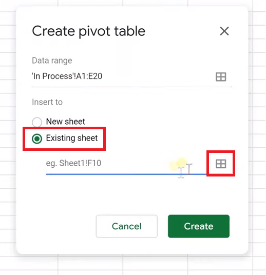
Select “Existing Sheet” and drop the table into G2 by
clicking the box to the right, then selecting G2.
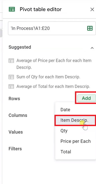
We’ll sort this by the sales quantity by item
description. Next to Rows in the Pivot Table Editor, click Add, and select Item
Description.
The Value will be “Quantity Sold.” We want this to be summed, so we will leave
this drop-down with the SUM value. This creates a simple table that sums the
sales by item description.
Create Another Pivot Table
To create the second Pivot Table, once again select Data then Pivot Table. We’ll use this table as a source and put this in G13. We’ll leave space because pivot tables expand and contract depending on what you do with them.
Second pivot table
First, we’ll add a row for the dates using the same method above, then right-click and group the dates. Go to “Create Pivot Date Group” and click “Month” for this example. We’ll do quantity again as the Value to populate the total sales for the items.
Date Group
This means we’ll need to add items to this second Pivot
Table, so we’ll drop in another row by clicking the Add button next to Row, and
selecting Item Description.
These two different tables are showing the same data in
different ways – one by item description and one by item description and date.
Filter – First Method
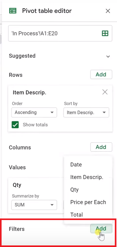
The first way to filter these Pivot Tables is to create normal filters that will act on both of these pivot tables as long as they are in the same sheet and working on the same data. Left-click on the Pivot Table, then go to the bottom of the editor to add a filter – let’s say to filter Item Description.
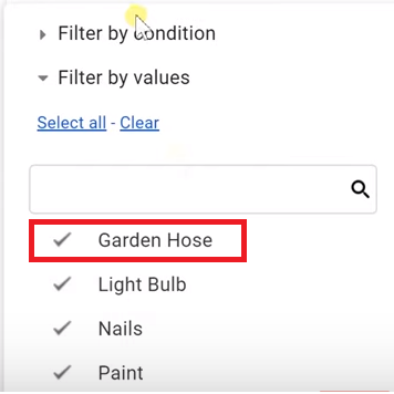
If you left-click on the status, you can either filter by condition or by values (which will be the same in the slicer). We’re going to take “garden hose” out.
Filters are specific to one pivot table. You won’t see this
being filtered unless you look at the options in the editor. If we remove the filter, Garden Hoses will
come back to the table. This means that no one will be able to see that this
data is being filtered unless they look at the editor. This also only applies
to one Pivot Table.
New Filter Option – Slicers
Instead of filters, we’re going to use Slicers and see how they operate differently. Go to Data then Slicer.
Now it’s asking for the data range. Click the original
table, not the pivot table, for the data range. We’re going to slice the source
data.
Drag the slicer over to the right. Since we’ve already selected the range, it automatically populates in the Slicer options. We’re going to skip the column for now, and we’re going to make sure that the checkbox is selected so that it applies to Pivot Tables.
In addition, you can further customize the slicer by
choosing different colors, fonts, etc. Let’s leave it the way it is.
Let’s filter by item description. We can only do one column
right now – if we need more, we’ll need to make additional Slicers.
The first thing we’re going to notice is that the Slicer is
already here for everyone to see. There are the same options to filter by
conditions and values when you click it. We’re going to do the same thing again
and filter out Garden Hose. Start by clicking the Filter icon on the left.
Add Another Slicer
The data still exists but is hidden. If we want to filter by
date, we will have to add an additional Slicer. All the Slicers on one sheet
have to work with the same ranges. Additionally, they are sheet specific, so
they will only filter the data on the original sheet.
The changes we have been making will only work in our user
profile with our sheet, so if you want these settings to apply to additional
users, you need to edit the slicer and pick “Set Current Filters as
Default” – that way they will see the same filters that you have.
Let’s continue filtering by date. We’re going to select date once again, and “Filter by Condition.” We only want it if it’s after August 1st, 2019. This table only has July values on it.
Before I click “okay” we can see that this table
has July values in it. When we update it, it will only have august.